5 Transformations

Transformations of predictors (and sometimes also of the outcome variable) are very common. There is nothing “fishy” about transformations - not transforming a predictor is as much a decision as making e.g. a log-transformation. The aim is not to conjure some non-existing effects. If a predictor shows an effect after transformation, this means that the nature of the relationship simply is on this transformed scale; if a predictor has a multiplicative effect on the outcome variable, we will find a linear relationship between the outcome variable and the log-transformed predictor. Without transformation, the model would violate the assumption of “identically distributed” data around the regression line, only the transformation makes the model valid.

When we use a transformation, we can still make effectplots (our favorite way to present the results) on the original scale. Or, we can plot on the transformed (e.g. log) scale; which one is better is not a statistical question, rather we should think about which version best conveys the biological (or other topical) meaning of our results.

We can distinguish two different types of transformations which have fundamentally different motivations and consequences.

Linear transformations

Linear transformations have no effect on the model performance itself: the variance explained by the model remains the same, effectplots don’t change. The motivation is not to achieve a better fit of the model to the data, but to a) facilitate model convergence and to b) improve the interpretability of model coefficients. The most commonly used linear transformation is centering and scaling (which can be called the “z-transformation”), for details see below. Complex models (e.g. those fitted with glmer, but often also simpler models) may not converge if you don’t apply a z-transformation to the linear predictors, especially when the predictor on the original scale has large values. For the same reason, when we want to include a polynomial term in the model, we usually use orthogonal rather than raw polynomials (polynomials are not linear transformations, but orthogonal polynomials are linear compared to raw polynomials). b) Coefficients of z-transformed predictors and of orthogonal polynomials have a more natural interpretation - discussed in the corresponding chapters below.

Non-linear transformations

The most commonly used non-linear transformations include the logarithm (usually just called log-transformation), polynomials (of degree 2 and more), the square-root, the arcussinus-squre-root (arcsin-square-root) and the logit. They have an effect on the model fit and will change the effectplot compared to using the untransformed predictor. E.g., when fitting a normal linear regression, the regression line will not be straight any more. The aim of these transformations is to improve model fit, i.e. to better capture the relationships that are in the data.

Non-linear transformations allow the use of the linear modeling framework even if the true nature of a relationship is not linear - to the degree that it can be represented by one of the available transformations. If the relationship is “very non-linear”, such as a complex phenology (activity of an organism over the year, with date as predictor), the effect of the predictor can be estimated using a smoother. In that case, we talk of a generalized additive model (GAM; actually, even GAM are linear models in their mathematical structure).

Note that transformations generally are only done for continuous predictors (= a covariable). However, sometimes, we may convert a (ordered) factor to a covariable, which can be seen as a type of transformation. This is discussed in a following chapter, together with the inverse: categorizing a covariable.

5.1 Some R-specific aspects

A transformation on a predictor can be calculated and stored as a new variable in the data object:

dat <- data.frame(a = runif(20,2,6),
                  b = rnorm(20,2,100))                           # some simulated data
dat$y <- rnorm(20,2-0.6*log(dat$a)-0.12*dat$b+0.003*dat$b^2,11)  # simulated outcome variable
dat$a.l <- log(dat$a)    # the log of x is stored in the new variable $x.l
dat$b.z <- scale(dat$b)  # the variable b is centerd and scaled to 1 SD by the function scale, and stored in $b.z

Then, the variable (“a.l”, “b.z”) can be used in the model just like any variable.

Alternatively, transformations can be done directly in the model formula:

mod1 <- lm(y ~ log(a), data=dat)     # the effect of the log of a on b is estimated
mod2 <- lm(y ~ b + I(b^2), data=dat) # using a linear and quadratic effect
  # as dat$b has large values, better use scaled dat$b, i.e. dat$b.z:
mod3 <- lm(y ~ b.z + I(b.z^2), data=dat)  # the I() makes that first the square is calculated, then these values are used
  # or, even better, especially for complex models, use orthogonal polynomials by applying the function poly
mod4 <- lm(y ~ poly(b,2), data=dat)   # the "2" asks for 2 polynomials, i.e. linear and quadratic

Models 2 to 4 are all the same model in the sense that they create the same effectplot.

Beware: It is often nice to z-transform the orthogonal polynomials. For that, we cannot use a double-function in the formula notation, rather the polynomials have to be created before the modeling, stored as a new variable, and only the z-transformation can be done in the formula (or outside, too, if you prefer). We get back to this in the polynomial chapter below.

mod5 <- lm(y ~ scale(poly(b,2)), data=dat)  # produces a wrong model!

5.2 First-aid transformations

J. W. Tukey termed the following three transformations the “first aid transformations”:

• log-transformation for concentrations and amounts
• square-root transformation for count data
• arcsin-square-root transformation for proportions (asin(sqrt(dat$x)))

Werner Stahel, a pivotal stats teacher for several of us, provides this information in his (german) book Stahel (2000). In our experience, the log-transformation can often be helpful, especially for strongly right skewed positive variables. We don’t often use the square-root transformation, but every now and then the arcsin-square-root transformation.

5.3 Log-transformation with Stahel

Log-transformations are often used and often very helpful, especially, as stated above, for strongly right skewed positive variables. Without the transformation, the large values, far away from the bulk of data, may have an unduely strong effect on the regression line (leading to a large “Cook’s distance”, see 12).

When log-transforming a predictor, we model its multiplicative effect on the outcome variable, while without transformation, it is the additive effect. This means: The model assumes that multiplying x by a factor F increases y by amount G (rather than increasing x by amount F increases y by amount G for the additive case). It seems that right skewed variables often relate in a multiplicative way to the outcome variable (for reasons that may lie in the heart of how mathematics works in our universe - we don’t know). But it is a good that down-scaling large values and changing to a multiplicative effect often both increase the model fit, else the log-transformation would not be that useful.

The log-transformation is great, as long as there are no zeros (and, of course, it does not work with negative values at all), as the log of 0 is minus infinity. But in real life, we often have zeros, and then, many people just add 1 to the values before log-transformation. This can be ok, but it is not optimal when the (non-zero) values are small. For that reason, some suggest to add 0.5 times the smallest non-zero value. Rob J Hyndman also presents the Box-Cox transformation in a blog, which apparently can be done using the R function log1p.

We made good experience with a transformation suggested by our above mentioned stats teacher Werner Stahel in his book (Stahel (2000), on p. 30): \(log(x + c)\), and c is the squared 25% quantile of the non-zero values divided by the 75% quantile of the non-zero values. This performs well with zeros, but is overall much better than adding 1 in many cases (and probably never worse).

set.seed(3)
x <- exp(runif(200,-3,5))  # a strongly skewed variable
x[sample(1:length(x),7)] <- 0   # put some values to exactly 0
x2 <- x/1000   # small values

# our custom function to calculate the Stahel-constant:
stahelc <- function(x) {
  ix <- x>0
  return((quantile(x[ix],0.25,na.rm=T))^2/quantile(x[ix],0.75,na.rm=T))
}

par(mfrow=c(2,4), mar=c(2,1,1,1), oma=c(0,2,1,0))
hist(x, nclass=30, main="raw values", xlab="", ylab="", yaxt="n")
mtext("larger values",2,1,xpd=NA)
hist(log(x+1), nclass=30, main="+1", xlab="", ylab="", yaxt="n")
hist(log(x+stahelc(x)), nclass=30, main="Stahel", xlab="", ylab="", yaxt="n")
hist(log1p(x), nclass=30, main="Box-Cox", xlab="", ylab="", yaxt="n")
hist(x2, nclass=30, main="raw values", xlab="", ylab="", yaxt="n")
mtext("small values",2,1,xpd=NA)
hist(log(x2+1), nclass=30, main="+1", xlab="", ylab="", yaxt="n")
hist(log(x2+stahelc(x2)), nclass=30, main="Stahel", xlab="", ylab="", yaxt="n")
hist(log1p(x2), nclass=30, main="Box-Cox", xlab="", ylab="", yaxt="n")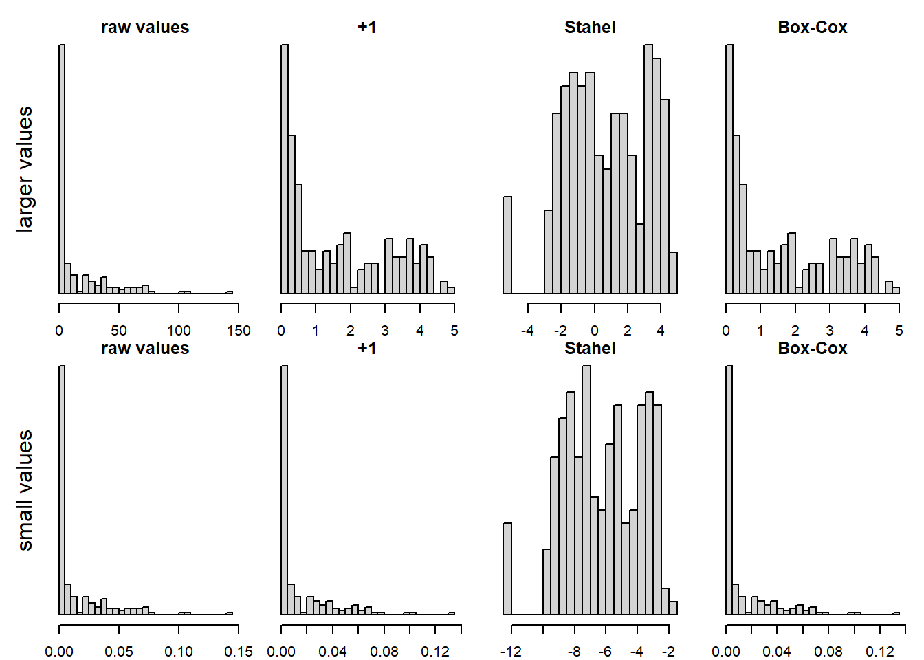

Figure 5.1: log-transformation of an original variable (leftmost two panels), for a variable with larger values (above row of panels) and one with smaller values (lower row). Adding 1 or the Box-Cox transformation don’t seem to help much, adding a constant according to Stahel performs best in these cases.

5.4 Centering and scaling (z-transformation)

Centering (\(x.c = x-mean(x)\)) is a transformation that produces a variable with a mean of 0. Centering is optional, but we have two good reasons reasons to center a predictor variable. First, it helps the model fitting algorithm to better converge because it reduces correlations among model parameters. Second, with centered predictors, the intercept and main effects in the linear model are better interpretable (they are measured at the center of the data instead of at the covariate value of 0 which may be far off).

Scaling: Scaling (\(x.s = x/c\), where \(c\) is a constant) is a transformation that changes the unit of the variable. Scaling is optional, too, but we have three good reasons to scale a covariable. First, to make the effect sizes better understandable. For example, a population change from one year to the next may be very small and hard to interpret. When we give the change for a 10-year period, its ecological meaning is better understandable. Second, to make the estimate of the effect sizes comparable between variables, we may use \(x.s = x/sd(x)\). The resulting variable has a unit of one standard deviation. A standard deviation may be comparable between variables that originally are measured in different units (meters, seconds etc). Andrew Gelman and Hill (2007) (p. 55 f) propose to scale the variables by two times the standard deviation (\(x.s = x/(2*sd(x))\)) to make effect sizes comparable between numeric and binary variables. Third, scaling can be important for model convergence, especially when polynomials are included. Also, consider the use of orthogonal polynomials, see below.

Centering and scaling to one standard deviation is usually done by the function scale:

dat$a.z <- scale(dat$a)  # using the arguments center and scale you can also only center or only scale
# this is the same as:
dat$a.z <- (dat$a - mean(dat$a)) / sd(dat$a)

5.5 Raw and orthogonal polynomials

Using polynomials allows to model some degree of non-linearity. The more polynomials are added, the more flexible becomes the curve to track data that has a non-linear relationship. However, in many cases we only add one polynomial - the quadratic effect - to the linear effect, sometimes also the cubic effect (i.e. the linear term is the first polynomial, the quadratic term the second and the cubic term the third polynomial). If you need more polynomials, a generalized additive model may be your better choice (though not always).

Raw polynomials are simply the original value squared, or raised to a higher power. It is very advisable in most cases to do that only on z-transformed values, as polynomials are quickly very large numbers, causing convergence problems. Also, polynomials are generally correlated, often strongly. This correlation is reduced if you use z-transformed values (at least for the correlation between linear and quadratic values), but there is (mostly) still a correlation there that may cause convergence problems in complex models. For this reason, we advise to use orthogonal polynomials using the function poly. Such polynomials are uncorrelated. Note: whether you use raw or orthogonal polynomials, the model performance is the same (the effecplot will look identical). But convergence is better with orthogonal polynomials, and also the interpretation of the coefficients: e.g. with two polynomials, the first coefficient captures the linear part of the relationship, the second the quadratic part.

We illustrate the use of polynomials in an example in Chapter 11.6. To summarize the points elaborated there:

• Adding polynomials adds flexibility to the model
• Quite often, we add the quadratic polynomial, sometimes the cubic, rarely higher-order polynomials
• Raw polynomials should generally be done on z-transformed values
• Orthogonal polynomials are uncorrelated and should be used in more complex models
• Orthogonal polynomials created with poly have small values, hence z-transforming them, too, can be advisable to make coefficient estimated comparable with other covariates

Quadratic polynomials are common in ecology because often, a relationship is not simply linear but has an optimum, e.g. of rainfall on growth - too little and too much rain are both not ideal for most plants. In such a case, the quadratic effect typically will be negative, because this means that the curve (= the regression line) has an optimum; a positive quadratic effect produces a curve that has a minimum. Of course, across the range of the predictor, we may only cover a part of the curve, hence a negative quadratic effect can also be a curve that increases and gradually levels off. This is typically seen for a species-area curve: as the size of a study plot increases, more species are found, but fewer and fewer new species can be added the more species are already in the pool of observed species. If we extrapolyte such a regression line beyond the maximal size of our study plots, the curve would start to decline, which is biological nonsense (in most cases!). Extrapolations of regression lines beyond the observed data are always delicate, but especially when polynomials are included.

dat <- data.frame(area = c(0.5,0.5,1,1,2,2.3,3,3.3,4,5,5.5),
                  species = c(2,3,4,5,6,6,7,8,7,8,9))
plot(dat$area, dat$species, las=1, xlab="Size of study area", ylab="Nr of species found",
     ylim=c(0,10),xlim=c(0,10))
mod <- lm(species ~ poly(area,2), data=dat)   # for species, a Poisson model would be a natural approach, but Gauss also works in our case
t.area <- seq(min(dat$area),max(dat$area),l=100)  # span 100 values across which to draw the regression line
lines(t.area, predict(mod, newdata = data.frame(area=t.area)), col="red")
# further extrapolytion would not make biologically sense here:
t.area <- seq(max(dat$area)+0.2,10,l=100)  # span 100 values across which to draw the regression line
lines(t.area, predict(mod, newdata = data.frame(area=t.area)), col="blue")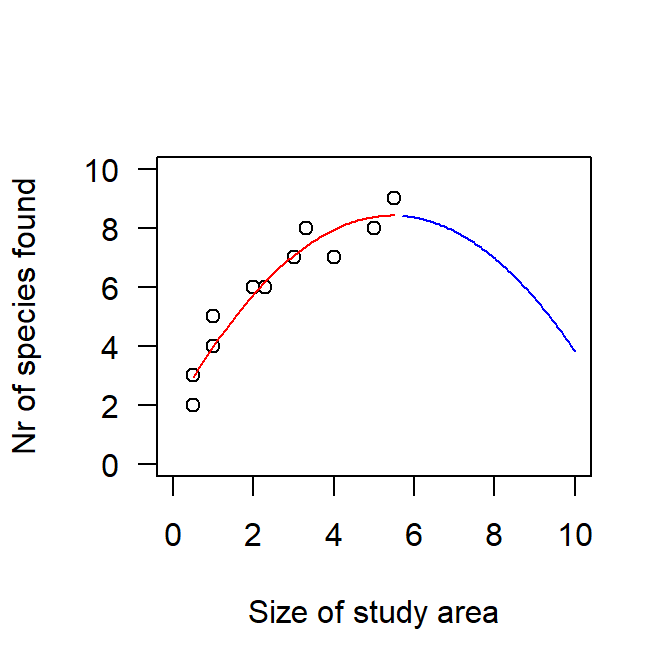

Figure 5.2: Observed relationship between the size of the study area and the number of species found there (circles) with a linear-quadratic regression line (red) to describe this relationship. While this line is a reasonable model for the data at hand, it is nonsense to extrapolate the line beyond the available data (blue line).

5.6 Square-root transformation

The square-root transformation is like a “mild” log-transformation and it has the advantage that zeros are not a problem. However, we rather rarely use it - it seems it often does not improve model fit much (or we don’t try often enough). Anyways, keep it in our toolbox!

5.7 Arcsinus-square-root transformation

The arccin-square-root transformation has been suggested for proportions. If you have the number of germinated seeds among a total number of seeds in the pot, you would use a binomial model (Chapter @glm and @glmm). But sometimes, you may only have the proportion that germinated, not the number and not the total, and, therefore, a binomial model is not possible. Then, the arcsin-square-root transformation can be a good choice. It stretches the effect at the ends, such that a change from 1% to 2% corresponds to a larger change than a change from 50% to 51%, which makes sense biologically in many or most cases (the first is a doubling, the second only a minor change).

The logit-transformation (see next chapter) has an analogous effect, but it cannot be applied to values of exactly 0 or 1, while arcsin-square-root does. The coefficient of a logit-transformed proportion has an interpretable meaning (albeit not a very easy one: see the discussion on odds ratios in Chapter 14), the coefficient of a arcsin-square-root transformation does not (except for the sign). But interpreting results works better looking at effectplots than coefficients anyways. So if you have 0s or 1s in the data, the arcsin-square-root is the better option than the logit; this is also true if you have values extremely close to 0 or 1, because the logit has a stronger effect on such values (as it goes towards minus/plus infinity at the extremes), potentially making these observations unduely influential; the arcsin-square-root transformation, on the other hand, does not go beyond 0 and (the meaningless valu of) 1.57:

asin(sqrt(c(0,1)))

## [1] 0.000000 1.570796

For values not at the extremes, arcsin-square-root and logit produce similar transformations.

5.8 Logit transformation

Above, we have already discussed the use of the logit-transformation for proportions, with the disadvantage that it does not work for the limit values of 0 and 1. Hence, it is actually not often used to transform predictors. However, it is used in (almost) all binomial models (to which Bernoulli models = logistic regressions belong, too) as the link function (see Chapter 14). For that reason, we here provide the formula: it is the log of the probability divided by one minus the probability:

\[ logit(p) = log(\frac{p}{1-p}) \]

The term inside the log is called the odds, hence the logit-transformation could also be called the log-odds-transformation.

In the packages loaded by R by default, there is no logit function. Surely, there are packages that do it, but it is not often needed. The inverse function of logit, however, is needed regularly: When you predict using the linear predictor of a binomial model, you get the estimated value on the logit-scale; you can then apply the inverse logit function plogis to get the estimate on the familiar probability scale.

5.9 Categorizing and decategorizing

Sometimes, none of the above transformations help to achieve a reasonably linear relationship between a covariate and the outcome variable. Then, a sensible solution can be to categorize the covariate and use it in the model as a factor. This can be a good choice e.g. when the covariable has many zeros, some small values and few large values: this could be categorized as “0”, “>0 to 1” and “>1”. How many levels you can make depends on the amount of data you have (more data allows for more levels) and the aim the model (are you mostly interested in zero vs non-zero, or also in finer classes?). Note that with each additional level, the model needs one more parameter (or more, if the predictor is also in interaction with other predictors).

In rather rare cases, it may also be reasonable to “decategorize” a factor, i.e. to use the factor levels as a covariate. This, of course, can only make sense for an ordered factor (i.e. the levels have a natural order). Also, going from one level to the next should have roughly the same effect on the outcome variable for all levels (if that is not the case, you would notice it in the residual analyses).

In R, you can use the function cut to categorize a covariate. Applying as.numeric to a factor will return the ranks of the factor levels, hence that can be used to turn an (ordered) factor into a covariate.

5.10 Sinus and cosinus transformation for circular variables

Variables like date (when spanning an entire year) or direction (in the sense of 0 to 360°, such as wind direction) are circular: the two ends (1 January and 31 December, 0° and 359°) are actually right next to each other. When you fit a simple linear regression to such data, e.g. the effect of wind direction on the number of migrants passing a study site, the two ends will not match (unless the line is horizontal), which makes no sense biologically. We can apply a sinus and cosinus transformation to match the two ends. The transformation has to be made on the radians, i.e. values from \(0\) to \(2\pi\), hence convert a julian day to \(day/365*2*\pi\), direction to \(direction/360*2*\pi\), etc.

set.seed(8)
dat <- data.frame(wind = sort(sample(0:359,120, replace = T)),
                  migration = as.numeric(mapply(function(x) rpois(10,x), x=c(15,10,5,2,2,6,9,15,20,32,25,20))))
dat$wind.n <- cos(dat$wind/360*2*pi)   # northwind component: 1 for perfect north, -1 for perfect south wind
dat$wind.e <- sin(dat$wind/360*2*pi)   # eastwind component: 1 for perfect east, -1 for perfect west wind
mod <- lm(migration ~ wind.n + wind.e, data=dat)
summary(mod)$coefficients[,c("Estimate","Std. Error")]

##              Estimate Std. Error
## (Intercept) 12.020347  0.4399101
## wind.n       7.943276  0.6712879
## wind.e      -8.967165  0.5775515

A positive effect of wind.n means that there is more migration the larger the northern component of the wind, a negative effect of wind.e means that there is less migration the larger the eastern component of the wind (and hence, more migration with more westerly winds).

Result interpretation is easier from an effectplot:

t.wind <- seq(0,365,l=100)   # prepare a sequence of wind-values for which to draw the regression line
t.wind.n <- cos(t.wind/365*2*pi)  # same transformation as before
t.wind.e <- sin(t.wind/365*2*pi)

par(mar=c(4,4,1,1))
plot(dat$wind, dat$migration, xlab="Winddirection\n(where wind comes from)",ylab="Migration activity",las=1, xaxt="n")
  # make a meaningful x-axis:
axis(1,at=seq(0,365,by=45),c("N","NE","E","SE","S","SW","W","NW","N"))
lines(t.wind, predict(mod, newdata=data.frame(wind.n=t.wind.n, wind.e=t.wind.e)), col="red",lwd=2)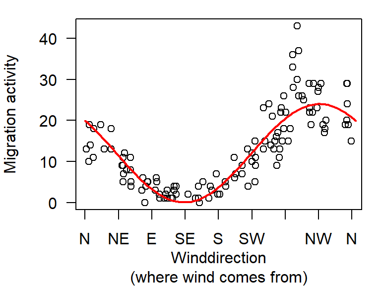

Figure 5.3: Relationship between wind direction and migration activity (circles; virtual data). We fit a linear regression through the data using two circular wind variables (north and east components).

Note: the two ends of the line match.

5.11 Cloglog, probit, inverse transformation

These transformations are not used often in ecology. They can e.g. be used as link functions in a binomial model, but usually, the logit-link function is used.

Note the risk for confusion of the term “inverse transformation”: here, it means \(f(x) = 1/x\), while in other contexts, it can mean “applying the inverse transformation of the transformation that had been done”, e.g. using \(exp()\) on a outcome variable that was log-transformed; if you use “back-transformation” in this context, there is no risk of confusion (but “apply the inverse link function” is often used in the context of binomial models, Chapter 14).

5.12 Identity transformation

This simply means the transformation to itself, i.e. no transformation. We only list this here because, sometimes, we read about the “identity link” in the context of generalize linear models (Chapter 14), where a link function is used (e.g. log-link function for Poisson models). Normal linear models (11) are a special case of generalize linear models, namely a Gauss (or “normal”) model with an identity-link function.

5.13 Transformations on the outcome variable

Transformations can also be made on the outcome variable. A very skewed outcome variable may be log-transformed. If the outcome variable is a proportion (e.g. the proportion of survivors from a nest, and we don’t have the actual number of survivors and non-survivors - if we have these numbers, we would fit a binomial model 14), the arcsin-square-root transformation can be meaningful.

But remember to back-transform predictions, if you want to give them on the original scale!

5.14 Back-transformation

In many contexts we want to back-transform a transformed value to its original value. This is especially common in generalized linear (mixed) models, where the prediction from the linear predictor is on the link scale (log for Poisson and negative-binomial models, logit for binomial models; see Chapter 14). In suche cases, we apply the “inverse link function” (i.e. doing the back-transformation) to get the values on the original scale. Hence, predictions from a Poisson model are exp-transformed to get the estimates (or predicted value) of the outcome variable on its original scale (e.g. number of individuals); predictions from a binomial model are inverse-logit-transformed (function plogis) to get the estimate ot he original scale (i.e. a probability in the case of a binomial model). Note that depending on the R function you use, this back-transformation is done automatically, e.g. when using predict with argument tpye=response, or when using posterior_epred (applied to a model fitted with rstanarm or brms, Chapter 11.1.2.4).

A technical note: you can get the inverse link-function to a model you fitted using the function family; it works with models fitted with glm, but may be others, too, depending on whether the package authors have implemented this. You apply the function family to the fitted model and extract the $lininv from that, which is the inverse link function:

m <- glm(c(1,1,1,0,0,0,1,1,1,0)~runif(10,3,7), family=binomial)  # default link function is logit
family(m)$linkinv(3)   # inverse link of logit; is the same as plogis:

## [1] 0.9525741

plogis(3)

## [1] 0.9525741

m <- glm(c(1,1,1,0,0,0,1,1,1,0)~runif(10,3,7), family=binomial(probit))  # alternative link function: probit
family(m)$linkinv(3)   # inverse probit function

## [1] 0.9986501

5.15 Applying the transformations to new data

Often, we want to predict from a model. This means: we define values for all predictors in the model and the predict the outcome value for these predictor values. This is done when we are interested in a specific scenario of predictor values, and we do it extensively when creating effectplots that depict the relationship between the outcome variable and a predictor.

When we want to predict for specific values of the predictors, we usually store these values in an object called “newdat”, because the values are like new data (for which we want to estimate the value of the outcome variable). We can then use “newdat” to make the effectplot. Hence, in newdat, we need the predictor values on their original scale (so that the effectplot is easy to interpret). But we also need the predictors on the scale used in the model - for making the prediction. Our approach is to create the “newdat” using values on the original scale.

For example, in the circual variables chapter above, we created 100 values from the minimum to the maximum of the observed wind values. We then predicted for each of these to be able to draw the effectplot. But to be able to predict, we also needed the new (100) wind values on the scale used in the model, i.e. the cosinus- and sinus-transformed values.

Care has to be taken when applying the same transformation that was used on the original variable (e.g. called dat$x) again on the variable in a new dataframe, e.g. on newdat$x: When the transformation depends on a statistic of the original dat$x, e.g. on \(mean(dat\$x)\), we also have to use \(mean(dat\$x)\) and not \(mean(newdat\$x)\) for the transformation done on newdat$x. Table 5.1 shows which transformation to use on newdat$x for a given transformation used on the original variable. Note the use of dat$x (rather than newdat$x) in the newdat-transformations for log with Stahel, center, scale, z, and orthogonal poly.

Table 5.1: Transformations more or less regularly used on covariates (sometimes also on the outcome variable), here, as an example, on dat$x, and how the transformation must be done when creating a “newdat” with newdat$x to then be used to predict from the model. “Stahel” stands for the constant proposed by W. Stahel (see chapter on log above). For the logit-transformation, only probabilities are possible (hence the dat$p), for sinus and cosinus only radians (hence the dat$r).

transformation	transformation done on dat$x	transformation done on newdat$x
log	log(dat$x)	log(newdat$x)
log + 1	log(dat$x+1)	log(newdat$x+1)
log with Stahel	log(dat$x+stahelc(dat$x))	log(newdat$x+stahelc(dat$x))
center	dat$x - mean(dat$x)	newdat$x - mean(dat$x)
scale to 1 SD	dat$x / sd(dat$x)	newdat$x / sd(dat$x)
z	scale(dat$x)	(newdat$x - mean(dat$x)) / sd(dat$x)
raw poly	dat$x^2, dat$x^3, etc	newdat$x^2, newdat$x^3, etc
orthogonal poly (e.g. 2)	poly(dat$x,2)	predict(poly(dat$x,2), newdata=newdat$x)
square-root	sqrt(dat$x)	sqrt(newdat$x)
asin-square-root	asin(sqrt(dat$x))	asin(sqrt(newdat$x))
logit	log(dat$p / (1-dat$p))	log(newdat$p / (1-newdat$p))
sin	sin(dat$r)	sin(newdat$r)
cosin	cos(dat$r)	cos(newdat$r)