12 Assessing model assumptions
12.1 Model assumptions
Every statistical model makes assumptions. We try to build models that reflect the data-generating process as realistically as possible. However, a model never is the truth. Yet, all inferences drawn from a model, such as estimates of effect size or derived quantities with credible intervals, are based on the assumption that the model is true. However, if a model captures the data generating process poorly, for example, because it misses important structures (predictors, interactions, polynomials), inferences drawn from the model are probably biased and results become unreliable. In a (hypothetical) model that captures all important structures of the data generating process, the stochastic part, the difference between the observation and the fitted value (the residuals), should only show random variation. Analyzing residuals is a very important part of the data analysis process.
Residual analysis can be very exciting, because the residuals show what remains unexplained by the present model. Residuals can sometimes show surprising patterns and, thereby, provide deeper insight into the system. However, at this step of the analysis it is important not to forget the original research questions that motivated the study. Because these questions have been asked without knowledge of the data, they protect against data dredging. Of course, residual analysis may raise interesting new questions. Nonetheless, these new questions have emerged from patterns in the data, which might just be random, not systematic, patterns. The search for a model with good fit should be guided by thinking about the process that generated the data, not by trial and error (i.e., do not try all possible variable combinations until the residuals look good; that is data dredging). All changes done to the model should be scientifically justified. Usually, model complexity increases, rather than decreases, during the analysis.
12.2 Independent and identically distributed
Usually, we model an outcome variable as independent and identically distributed (iid) given the model parameters. This means that all observations with the same predictor values behave like independent random numbers from the identical distribution. As a consequence, residuals should look iid. Independent means that:
The residuals do not correlate with other variables (those that are included in the model as well as any other variable not included in the model).
The residuals are not grouped (i.e., the means of any set of residuals should all be equal).
The residuals are not autocorrelated (i.e., no temporal or spatial autocorrelation exist; Sections 12.4 and 12.5).
Identically distributed means that:
- All residuals come from the same distribution.
In the case of a linear model with normal error distribution (Chapter 11) the residuals are assumed to come from the same normal distribution. Particularly:
The residual variance is homogeneous (homoscedasticity), that is, it does not depend on any predictor variable, and it does not change with the fitted value.
The mean of the residuals is zero over the whole range of predictor values. When numeric predictors (covariates) are present, this implies that the relationship between x and y can be adequately described by a straight line.
Residual analysis is mainly done graphically. R makes it easy to plot residuals to look at the different aspects just listed. As an example, we use a linear regression for the biomass of the grass species Dactylis glomerata in relation to water conditions in the soil.
The first panel in Fig. 12.1 shows the residuals against the fitted values together with a smoother (red line). This plot is called the Tukey-Ascombe plot. The mean of the residuals should be around zero along the whole range of fitted values. Note that smoothers are very sensitive to random structures in the data, especially for low sample sizes and toward the edges of the data range. Often, curves at the edges of the data do not worry us because the edges of smoothers are based on small sample sizes.
The second panel a normal quantile-quantile (QQ) plot of the residuals. When the residuals are normally distributed, the points lie aong the diagonal line. This plot is explained in more detail below.
The third panel shows the square root of the absolute values of the standardized residuals, a measure of residual variance, versus the fitted values, together with a smoother. When the residual variance is homogeneous along the range of fitted values, the smoother is horizontal.
The fourth panel shows the residuals against the leverage. An observation with a measurement of a predictor variable far from the others has a large leverage. When all predictors are factors, observations with a rare combination of factor levels have higher leverages than observations with a common combination of factor levels. Such observations have the potential to have a large influence on the regression line. A high leverage does not necessarily mean that this observation has a big influence on the model. If that observation fits well to the pattern of all other data points, the observation does not have an unduly large influence on the model estimates, despite its large leverage. However, if it does not fit into the picture, this observation has a strong influence on the parameter estimates.
The influence of one observation on the parameter estimates is measured by the Cook’s distance. Observations with large Cook’s distances lie beyond the red dashed lines in the fourth of the residual plots (the 0.5 and 1 iso lines for Cook’s distances are given as dashed lines). Observations with a Cook’s distance larger than 1 are usually considered to be overly influential and should be checked.
The diagnostic plots (Fig. 12.1) of the residuals of the model fitted to the data of the species Dactylis glomerata look quite acceptable. 1. The average residual value is around zero along the range of fitted values, 2. the points are alined diagonally in the QQ-plot, 3. the variance does not noticably change along the fitted values, and 4. no observation has a large Cook’s distance.
data(ellenberg)
mod <- lm(Yi.g~Water, data=ellenberg[ellenberg$Species=="Dg",])
par(mfrow=c(2,2))
plot(mod)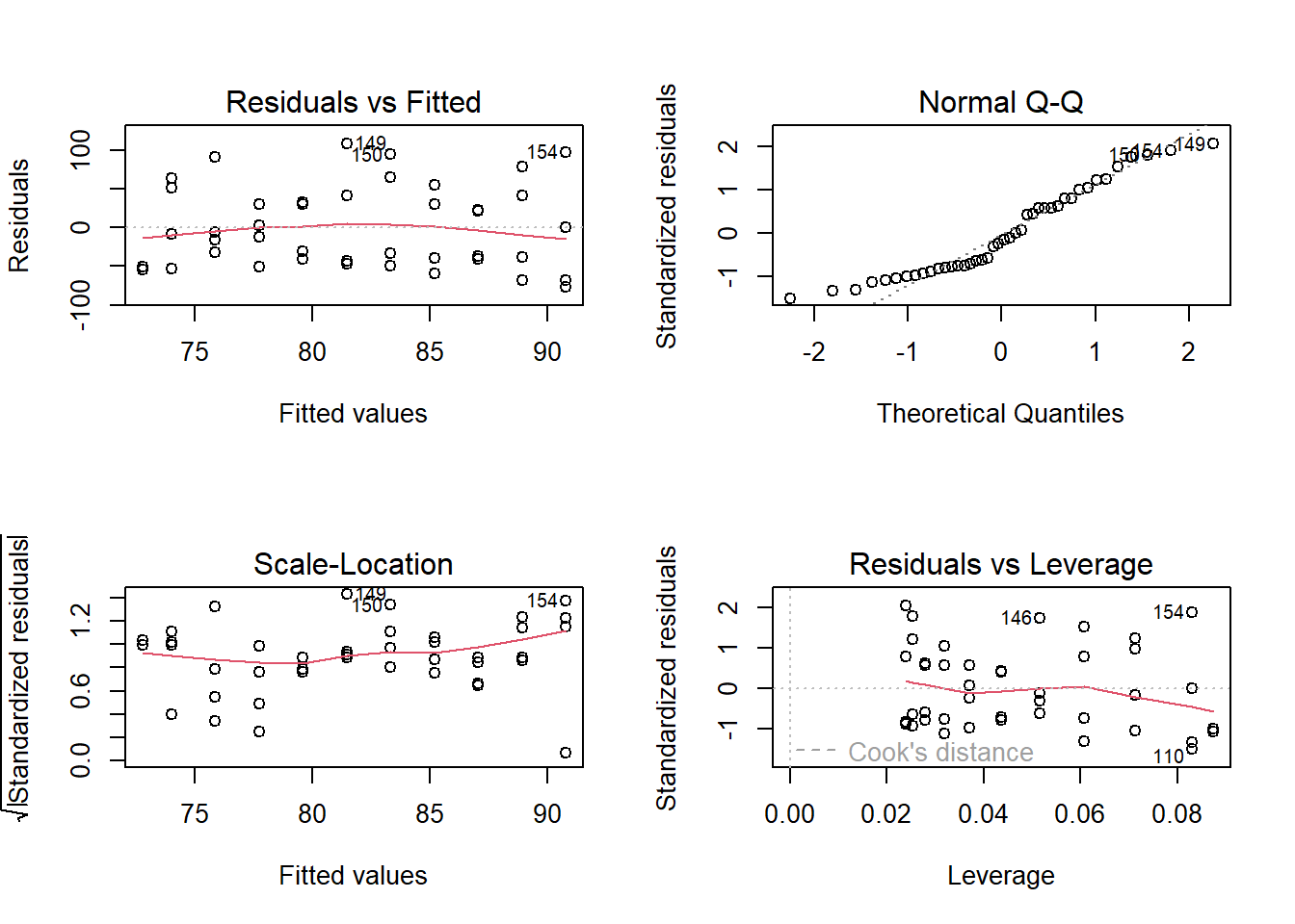
Figure 12.1: Standard diagnostic residual plots of a linear regression for the biomass data of D. glomerata.
However, when the same model is fitted to data of Alopecurus pratensis, the model assumptions may not be met well (Fig. 12.2). The average of the residuals decreases with increasing fitted values (panel 1). A few observations, in particular observation 133, do not fit to a normal distribution (panel 2). The residual variance increases with increasing fitted values (panel 3). Observation 133 has a too high Cook’s distance.
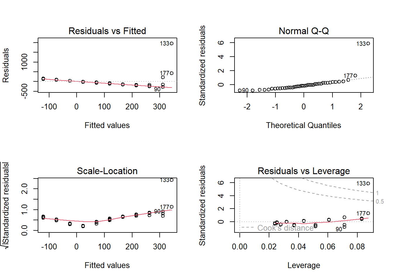
Figure 12.2: Standard diagnostic residual plots of a linear regression for the biomass data of A. pratensis.
An increasing variance with increasing fitted values is a widespread case. The logarithm or square-root transformation of the response variable often is a quick and simple solution. Also, in this case, the log transformation improved the diagnostic plots (Fig. 12.3).
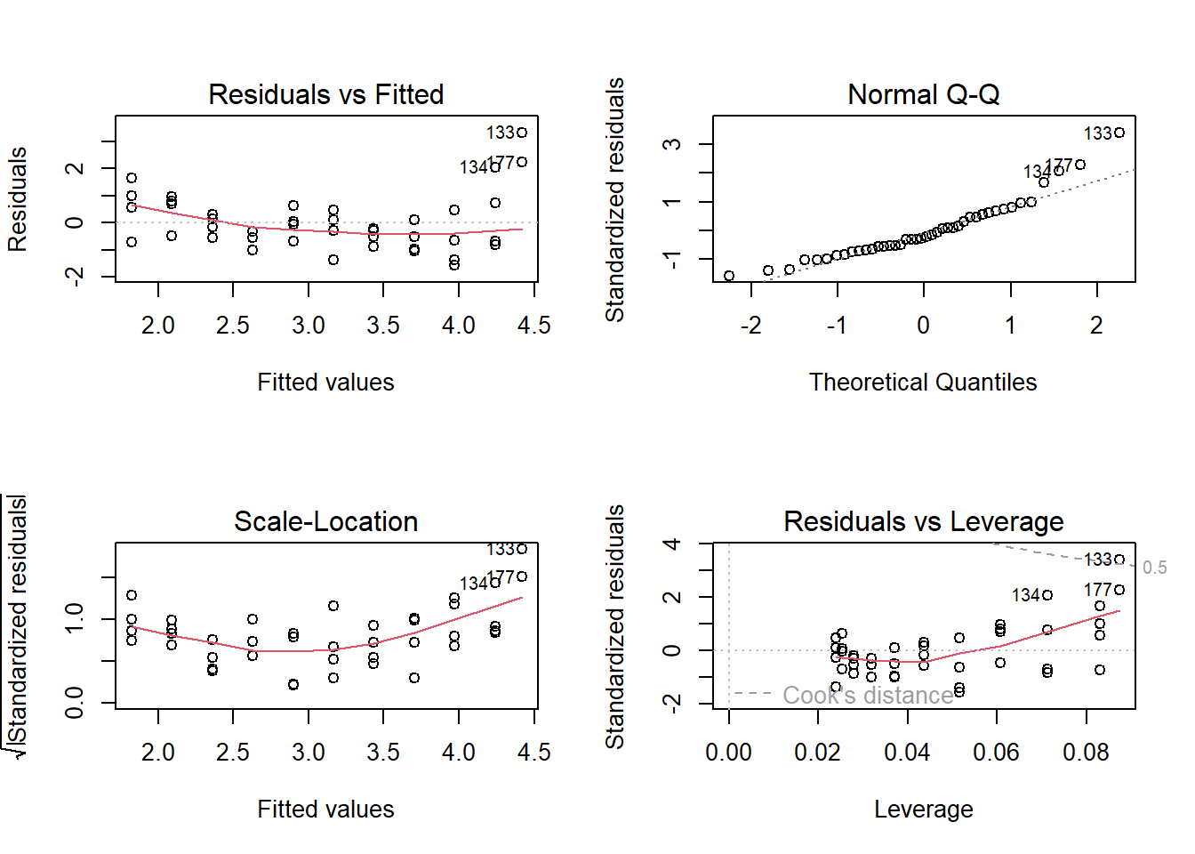
Figure 12.3: Standard diagnostic residual plots of a linear regression for the logarithm of the biomass data of A. pratensis.
The four plots produced by plot(mod) show the most important aspects of the model fit. However, often these four plots are not sufficient. IN addition, we recommend plotting the residuals against all variables in the data set (including those not used in the current model). It is further recommended to think about the data structure. Can we assume that all observations are independent of each other? May there be spatial or temporal correlation?
12.3 The QQ-plot
Each residual represents a quantile of the sample of \(n\) residuals. These quantiles are defined by the sample size \(n\). A useful choice is the \(((1,...,n)-0.5)/n\)-th quantiles. A QQ-plot shows the residuals on the y-axis and the values of the \(((1,...,n)-0.5)/n\)-th quantiles of a theoretical normal distribution on the x-axis. A QQ-plot could also be used to compare the distribution of whatever variable with any distribution, but we want to use the normal distribution here because that is the assumed distribution of the residuals in the model. If the residuals are normally distributed, the points are expected to lie along the diagonal line in the QQ-plot.
It is often rather difficult to decide whether a deviation from the line is tolerable or not. The function compareqqnorm may help. It draws, eight times, a random sample of \(n\) values from a normal distribution with a mean of zero and a standard deviation equal to the residual standard deviation of the model. It then creates a QQ-plot for all eight random samples and for the residuals in a random order. If the QQ-plot of the residuals can easily be identified amont the nine QQ-plots, there is reason to think the distribution of the residuals deviates from normal. Otherwise, there is no indication to suspect violation of the normality assumption. The position of the residual plot of the model in the nine panels is printed to the R console.