18 MCMC using Stan via rstanarm, brms or rstan

18.1 Background

Markov chain Monte Carlo (MCMC) simulation techniques were developed in the mid-1950s by physicists (Metropolis et al., 1953). Later, statisticians discovered MCMC (Hastings, 1970; Geman & Geman, 1984; Tanner & Wong, 1987; Gelfand et al., 1990; Gelfand & Smith, 1990). MCMC methods make it possible to obtain posterior distributions for parameters and latent variables (unobserved variables) of complex models. In parallel, personal computer capacities increased in the 1990s and user-friendly software such as the different programs based on the programming language BUGS (Spiegelhalter et al., 2003) came out. These developments boosted the use of Bayesian data analyses, particularly in genetics and ecology.

In this book we use the program Stan to draw random samples from the joint posterior distribution of the model parameters given a model, the data, prior distributions, and initial values. To do so, it uses the “no-U-turn sampler,” which is a type of Hamiltonian Monte Carlo simulation (Hoffman and Gelman 2014; M~J Betancourt 2013), and optimization-based point estimation. These algorithms are more efficient than the ones implemented in BUGS programs and they can handle larger data sets. Stan works particularly well for hierarchical models (Michael Betancourt 2013). Stan runs on Windows, Mac, and Linux and can be used via the R interfaces (package) rstanarm, brms or rstan. Stan is automatically installed when one of these R-packages is installed.

According to our experience, rstanarm can be installed from CRAN as any R-package without problems. With brm, sometimes, it has been a bit more difficult. You should use a recent version of R and RStudio (if you use that). It seems advisable to first install Rtools (for Windows) or Xcode (for Mac). Search the web for instructions to do that (RTools is a program, not an R package; it is installed directly on C:, by default). Then, brms can be installed in the normal way within R using install.packages. rstan should be installed automatically, else install it following online instructions here.

A trick that helped more than once when we had problems to run brm was:

# after installing or updating brms, the got warnings regarding "make not found" and MCMC
# sampling did not start. The following may help (solution found here:
# https://discourse.mc-stan.org/t/error-when-running-brm-model/27951) 

# after installing rtools, rstan and brms, run this in the console:
remove.packages(c("StanHeaders", "rstan"))
 # may give a warning if you don’t have StanHeaders, but that’s ok
install.packages("StanHeaders", repos = c("https://mc-stan.org/r-packages/", getOption("repos")))
install.packages("rstan", repos = c("https://mc-stan.org/r-packages/", getOption("repos")))

An alternative to rtools may be to use brm together with the package cmdstanr, but we have only limited experience so far.

18.2 Assessing convergence of the Markov chains and trouble shooting warnings of Stan

The MCMC sampling is not guaranteed to converge, and/or the returned samples may be autocorrelated to a degree that your effective number of draws from the joint posterior is nowhere near 4000, the number of draws returned by default from brm. For simple models like a linear regression, there will not generally be a problem, but for more complex models, issues about the validity of the returned draws appear quite regularly.

We first check whether we find warnings in the R console about problems of the fitting algorithm. Warnings should not simply be ignored. Often, we find help in the Stan online documentation (or when typing launch_shinystan(mod.brm) into the R-console) what to change. Some points from our applied experience, especially regarding fitting models with brm:

When you get warnings, first of all make sure you help the algorithm as much as possible:
- center and scale (to 1 SD) continuous predictors
- use orthogonal polynomials
- reduce model complexity
- reduce sparse factor levels (aggregate with other levels or omit such observations)
- treat factors with many levels as random factors, or, if appropriate, as continuous predictors (if levels are clearly ordered)
Probably the most common warning is about “divergent transitions”. Ideally, the problem is resolved by re-parametrizing the model, but that’s probably often not possible. One suggestion is to increase the “adapt delta” using the argument control = list(adapt_delta = 0.99) in the brm function. This will increase the fitting time and can resolve the problem, but not always. In our experience, if ESS and R-hat (see below) are fine, getting rid of some or all divergent transitions by increasing adapt delta generally does not change parameter estimates much. While the math cracks say that divergent transition warnings should be taken seriously (link), in our experience, the model may be ok even with some 100 divergent transitions, if and only if R-hat and ESS are fine. But be cautious about this!
The warning about “exceeding maximum treedepth” is, according to the web source given above, less of a problem. It is about efficiency, not convergence. If R-hat and ESS are good, maximum treedepth warnings can probably be ignored.
Warnings about too high R-hat and/or too low ESS must be addressed in all cases. These warnings tell us that the model or parts of it have not converged and anything concluded from these draws may be complete nonsense. Often, the problem can be resolved by increasing the number of iterations, e.g. iter=20000. ESS warnings indicate that your MCMC draws are autocorrelated (thereby reducing the effective sample size ESS of your number of draws). Hence, in addition to increasing the number draws, you may want to thin the chains to prevent generating a lot of redundant numbers, e.g. thin=5. R-hat is a measure of convergence of chains; a R-hat of 1 means perfect mixing of chains and, hence, convergence, larger values indicate non-convergence (it’s good to have all R-hat <1.1, but larger values are accepted depending on the aim of the model). Generally, we get one R-hat value and two ESS values per estimated parameter.The two ESS values are “bulk ESS” and “tail ESS”. The first tells us about how many effectively independent draws we have in the middle of the marginal posterior distribution of the parameter. This should be >200 or better >2000. The tail ESS is about the effective number of draws in the two tails of the posterior, which is relevant for the quality of the compatibility interval estimate because this is defined as the 2.5% to 97.5% quantile of the posterior (which obviously are in the tails of the posterior). Again, it should probably be >200 or better >2000. Note that, as said, R-hat and ESS are given per parameter. If all values are fine but one or few parameters of little interest (e.g. a random effect level you are not much interested in) show R-hat of >1.1 and rather small ESS, and increasing the iterations does not help, you may still be content with the model, but you would not make great conclusions from the random effect levels that converged poorly.

R-hat and ESS are returned when you type the model object, or request the summary of it (see below), but for random levels, they may not all appear. You can get all values using this code:

library(brms)
library(posterior)

# load a model that has been fitted using brm
load("RData/mod.brm.compiled.RData")
mod.brm <- update(mod.brm.compiled, recompile = FALSE, seed=123, refresh=0)

apply(as.matrix(mod.brm), 2, rhat)

## b_Intercept         b_x       sigma   Intercept      lprior        lp__ 
##   1.0003384   1.0011481   1.0007055   0.9998799   1.0001323   1.0007838

apply(as.matrix(mod.brm), 2, ess_bulk)

## b_Intercept         b_x       sigma   Intercept      lprior        lp__ 
##    3810.513    3902.531    4183.216    4292.089    3780.433    1965.951

apply(as.matrix(mod.brm), 2, ess_tail)

## b_Intercept         b_x       sigma   Intercept      lprior        lp__ 
##    2575.402    2664.881    3097.737    3117.777    2721.946    2305.481

When we have no warnings, Markov chains likely have mixed well. Still, we should, at least for more complex models, check the mixing. We can either do that by scanning through the many diagnostic plots given by launch_shinystan(mod.brm), or create the most important plots ourselves such as the traceplot (Figure 18.1).

par(mar=c(2,2,2,2))
mcmc_plot(mod.brm, type = "trace")

Traceplot of the Markov chains. After convergence, the Markov chains should sample from the same stationary distribution. Indications of non-convergence would be if the chains diverge or vary around different means.

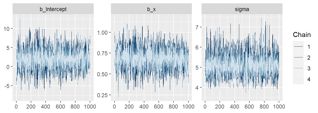
Figure 18.1: Traceplot of the Markov chains. After convergence, the Markov chains should sample from the same stationary distribution. Indications of non-convergence would be if the chains diverge or vary around different means.

18.3 Using Stan via rstan

18.3.1 Writing a Stan model

The statistical model is written in the Stan language and saved in a text file. The Stan language is rather strict, forcing the user to write unambiguous models. Stan is very well documented and the Stan Documentation contains a comprehensive Language Manual, a Wiki documentation and various tutorials.

We here provide a normal regression with one predictor variable as a worked example. The entire Stan model is as following (saved as linreg.stan)

data {
  int<lower=0> n;
  vector[n] y;
  vector[n] x;
}

parameters {
  vector[2] beta;
  real<lower=0> sigma;
}

model {
  //priors
  beta ~ normal(0,5);
  sigma ~ cauchy(0,5);
  // likelihood
  y ~ normal(beta[1] + beta[2] * x, sigma);
}

A Stan model consists of different named blocks. These blocks are (from first to last): data, transformed data, parameters, trans- formed parameters, model, and generated quantities. The blocks must appear in this order. The model block is mandatory; all other blocks are optional.

In the data block, the type, dimension, and name of every variable has to be declared. Optionally, the range of possible values can be specified. For example, vector[N] y; means that y is a vector (type real) of length N, and int<lower=0> N; means that N is an integer with nonnegative values (the bounds, here 0, are included). Note that the restriction to a possible range of values is not strictly necessary but this will help specifying the correct model and it will improve speed. We also see that each line needs to be closed by a column sign. In the parameters block, all model parameters have to be defined. The coefficients of the linear predictor constitute a vector of length 2, vector[2] beta;. Alternatively, real beta[2]; could be used. The sigma parameter is a one-number parameter that has to be positive, therefore real<lower=0> sigma;.

The model block contains the model specification. Stan functions can handle vectors and we do not have to loop over all observations as typical for BUGS . Here, we use a Cauchy distribution as a prior distribution for sigma. This distribution can have negative values, but because we defined the lower limit of sigma to be 0 in the parameters block, the prior distribution actually used in the model is a truncated Cauchy distribution (truncated at zero). In Chapter 10.2 we explain how to choose prior distributions.

Further characteristics of the Stan language that are good to know include: The variance parameter for the normal distribution is specified as the standard deviation (like in R but different from BUGS, where the precision is used). If no prior is specified, Stan uses a uniform prior over the range of possible values as specified in the parameter block. Variable names must not contain periods, for example, x.z would not be allowed, but x_z is allowed. To comment out a line, use double forward-slashes //.

Finally, the R-package brms provides the function make_stancode that translates an R-code of a model into Stan code. This can be a great starting point for your specific model.

18.3.2 Run Stan from R using rstan

We fit the model to simulated data. Stan needs a vector containing the names of the data objects. In our case, x, y, and N are objects that exist in the R console.

The function stan() starts Stan and returns an object containing MCMCs for every model parameter. We have to specify the name of the file that contains the model specification, the data, the number of chains, and the number of iterations per chain we would like to have. The first half of the iterations of each chain is declared as the warm-up. During the warm-up, Stan is not simulating a Markov chain, because in every step the algorithm is adapted. After the warm-up the algorithm is fixed and Stan simulates Markov chains.

library(rstan)

# Simulate fake data 
n <- 50                                      # sample size
sigma <- 5                                   # standard deviation of the residuals
b0 <- 2                                      # intercept
b1 <- 0.7                                    # slope

x <- runif(n, 10, 30)                        # random numbers of the covariate
simresid <- rnorm(n, 0, sd=sigma)            # residuals

y <- b0 + b1*x + simresid                    # calculate y, i.e. the data

# Bundle data into a list 
datax <- list(n=length(y), y=y, x=x)

# Run STAN
fit <- stan(file = "stanmodels/linreg.stan", data=datax, verbose = FALSE, refresh=0)

Bayesian Data Analysis in Ecology with R and Stan