9 The Bayesian paradigm and likelihood in a frequentist and Bayesian framework

9.1 Short historical overview

Reverend Thomas Bayes (1701 or 1702 - 1761) developed the Bayes theorem. Based on this theorem, he described how to obtain the probability of a hypothesis given an observation, that is, data. However, he was so worried whether it would be acceptable to apply his theory to real-world examples that he did not dare to publish it. His methods were only published posthumously (Bayes 1763). Without the help of computers, Bayes’ methods were applicable to just simple problems.
Much later, the concept of null hypothesis testing was introduced by Ronald A. Fisher (1890 - 1962) in his book Statistical Methods for Research Workers (Fisher 1925) and many other publications. Egon Pearson (1895 - 1980) and others developed the frequentist statistical methods, which are based on the probability of the data given a null hypothesis. These methods are solvable for many simple and some moderately complex examples.
The rapidly improving capacity of computers in recent years now enables us to use Bayesian methods also for more (and even very) complex problems using simulation techniques Gilks, Richardson, and Spiegelhalter (1996).

9.2 The Bayesian way

Bayesian methods use Bayes’ theorem to update prior knowledge about a parameter with information coming from the data to obtain posterior knowledge. The prior and posterior knowledge are mathematically described by a probability distribution (prior and posterior distributions of the parameter). Bayes’ theorem for discrete events says that the probability of event $A$ given event $B$ has occurred, $P(A|B)$, equals the probability of event $A$, $P(A)$, times the probability of event $B$ conditional on $A$, $P(B|A)$, divided by the probability of event $B$, $P(B)$: \[ P(A|B) = \frac{P(A)P(B|A)}{P(B)}\] When using Bayes’ theorem for drawing inference from data, we are interested in the probability distribution of one or several parameters, $\theta$ (called “theta”), after having looked at the data $y$, that is, the posterior distribution, $p(\theta|y)$. To this end, Bayes’ theorem is reformulated for continuous parameters using probability distributions rather than probabilities for discrete events: \[ p(\theta|y) = \frac{P(\theta)p(y|\theta)}{p(y)}\] The posterior distribution, $p(\theta|y)$, describes what we know about the parameter (or about the set of parameters), $\theta$, after having looked at the data and given the prior knowledge and the model. The prior distribution of $\theta$, $p(\theta)$, describes what we know about $\theta$ before having looked at the data. This is often very little but it can include information from earlier studies. The probability of the data conditional on $\theta$, $p(y|\theta)$, is called likelihood.

The word likelihood is used in Bayesian statistics with a slightly different meaning than it is used in frequentist statistics. The frequentist likelihood, $L(\theta|y)$, is a relative measure for the probability of the observed data given specific parameter values. The likelihood is a number often close to zero. In contrast, Bayesians use likelihood for the density distribution of the data conditional on the parameters of a model. Thus, in Bayesian statistics the likelihood is a distribution (i.e., the area under the curve is 1) whereas in frequentist statistics it is a scalar.

The prior probability of the data, $p(y)$, equals the integral of $p(y|\theta)p(\theta)$ over all possible values of $\theta$; thus $p(y)$ is a constant.

The integral can be solved numerically only for a few simple cases. For this reason, Bayesian statistics were not widely applied before the computer age. Nowadays, a variety of different simulation algorithms exist that allow sampling from distributions that are only known to proportionality (e.g., Gilks, Richardson, and Spiegelhalter (1996)). Dropping the term $p(y)$ in the Bayes theorem leads to a term that is proportional to the posterior distribution: $p(\theta|y)\propto p(\theta)p(y|\theta)$. Simulation algorithms such as Markov chain Monte Carlo simulation (MCMC) can, therefore, sample from the posterior distribution without having to know $p(y)$. A large enough sample of the posterior distribution can then be used to draw inference about the parameters of interest.

9.3 Likelihood

9.3.1 Theory

In Bayesian statistics the likelihood is the probability distribution of the data given the model $p(y|\theta)$, also called the predictive density. In contrast, frequentists use the likelihood as a relative measure of the probability of the data given a specific model (i.e., a model with specified parameter values). Often, we see the notation $L(\theta|y) = p(y|\theta)$ for thelikelihood of a model. Let’s look at an example. According to values that we found on the internet, black-tailed prairie dogs Cynomys ludovicianus weigh on average 1 kg with a standard deviation of 0.2 kg.

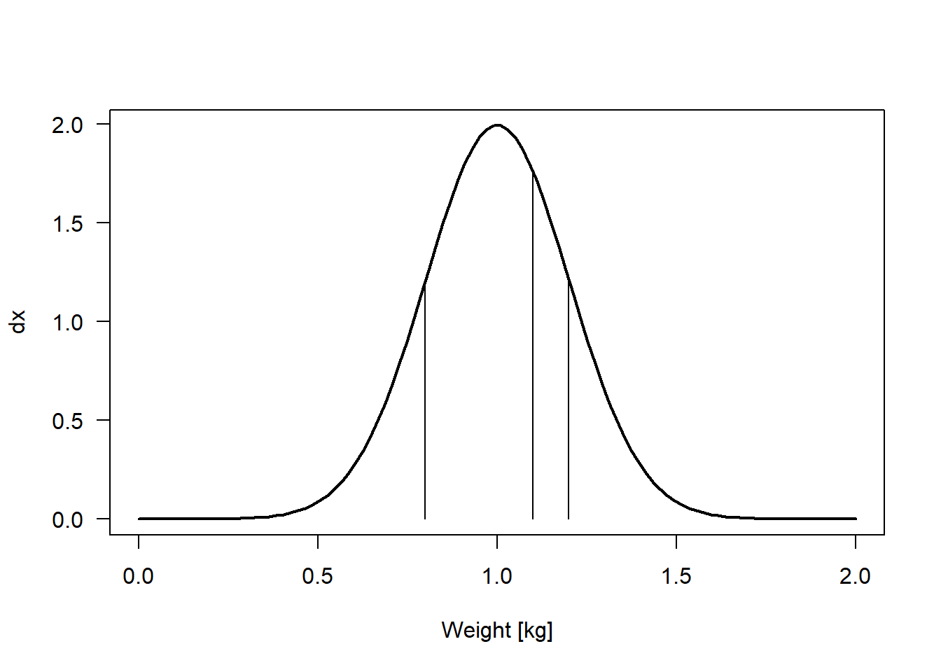
Using these values, we construct a model for the weight of prairie dogs $y_i \sim normal(\mu, \sigma)$ with $\mu$ = 1 kg and $\sigma$ = 0.2 kg. We then go to the prairie and catch three prairie dogs. Their weights are 0.8, 1.2, and 1.1 kg. What is the likelihood of our model given this data? The likelihood is the product of the density function (the Gaussian function with $\mu$ = 1 and $\sigma$ = 0.2) defined by the model and evaluated for each data point (Figure 9.1).

l <- dnorm(x=0.8, mean=1, sd=0.2)*dnorm(x=1.2, mean=1, sd=0.2)*
dnorm(x=1.1, mean=1, sd=0.2)
l

## [1] 2.576671

x <- seq(0,2, length=100)
dx <- dnorm(x, mean=1, sd=0.2)
plot(x, dx, type="l", lwd=2, las=1, xlab="Weight [kg]")
y <- c(0.8, 1.1, 1.2)
segments(y, dnorm(y, mean=1, sd=0.2), y, rep(0, length(y)))

Density function of a Gaussian (=normal) distribution with mean 1 kg and standard deviation 0.2 kg. The vertical lines indicate the three observations in the data. The curve has been produced using the function dnorm.

Figure 9.1: Density function of a Gaussian (=normal) distribution with mean 1 kg and standard deviation 0.2 kg. The vertical lines indicate the three observations in the data. The curve has been produced using the function dnorm.

The likelihood (2.6) does not tell us much. But, another web page says that prairie dogs weigh on average 1.2 kg with a standard deviation of 0.4 kg. The likelihood for this alternative model is:

l2 <-dnorm(x=0.8, mean=1.2, sd=0.4)*dnorm(x=1.2, mean=1.2, sd=0.4)*
dnorm(x=1.1, mean=1.2, sd=0.4)
l2

## [1] 0.5832185

Thus, the probability of observing the three weights (0.8, 1.2, and 1.1 kg) is four times larger given the first model than given the second model.
The normal density function is a function of $y$ with fixed parameters $\mu$ and $\sigma$. When we fix the data to value $y$ (i.e., we have a data file with $n = 1$) and vary the parameter, we get the likelihood function given the data and we assume the normal distribution as our data model. When the data contain more than one observation, the likelihood function becomes a product of the normal density function for each observation. \[ L(\mu, \sigma|y) = \prod_{i=1}^n p(y_i|\mu,\sigma) \] We can insert the three observations into this function.

y <- c(0.8, 1.2, 1.1)
lf <- function(mu, sigma) prod(dnorm(y, mean=mu, sd=sigma))

Applying the likelihood function to the model from the first web page, we get the following likelihood.

lf(1, 0.2)

## [1] 2.576671

9.3.2 The maximum likelihood method

A common method of obtaining parameter estimates is the maximum likelihood method (ML). Specifically, we search for the parameter combination from the likelihood function for which the likelihood is maximized. Also in Bayesian statistics, ML is used to optimize algorithms that produce posterior distributions (e.g., in the function sim).

To obtain ML estimates for the mean and standard deviation of the prairie dog weights, we calculate the likelihood function for many possible combinations of means and standard deviations and look for the pair of parameter values that is associated with the largest likelihood value.

mu <- seq(0.6, 1.4, length=100)
sigma <- seq(0.05, 0.6, length=100)
lik <- matrix(nrow=length(mu), ncol=length(sigma))
for(i in 1:length(mu)){
  for(j in 1:length(sigma)){
    lik[i,j] <- lf(mu[i], sigma[j])
  }
}
contour(mu, sigma, lik, nlevels=20, xlab=expression(mu),
ylab=expression(sigma), las=1, cex.lab=1.4) 

# find the ML estimates
neglf <- function(x) -prod(dnorm(y, x[1], x[2]))
MLest <- optim(c(0.5, 0.5), neglf) # the vector with numbers are the initial values


points(MLest$par[1],MLest$par[2], pch=13)

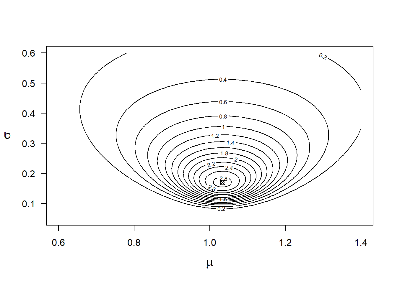
Figure 9.2: Likelihood function for y=0.8, 1.2, 1.1 and the data model y~normal(mu, sigma). The cross indicates the highest likelihood value.

MLest$par

## [1] 1.0333330 0.1699668

We can get the $\mu$ and $\sigma$ values that produce the largest likelihood by the function optim. This function finds the parameter values associated with the lowest value of a user defined function. Therefore, we define a function that calculates the negative likelihood.

The combination of mean = 1.03 and standard deviation = 0.17 is associated with the highest likelihood value (the “mountain top” in Figure 9.2). In the case of models with more than two parameters, the likelihood function cannot be visualized easily. Often, some parameters are fixed to one value, for example, their ML estimate, to show how the likelihood function changes in relation to one or two other parameters.

Likelihoods are often numbers very close to zero, especially when sample size is large. Then, likelihood values drop below the computing ability of computers (underflow). Therefore, the logarithm of the likelihood is often used. In addition, many standard optimizers are, in fact, minimizers such that the negative log-likelihood is used to find the ML estimates.

The ratio between the likelihoods of two different models - for example, $L(= 1, = 0.2|y)/L(= 1.2, = 0.4)|y) = 2.58/0.58 = 4.42 - is called the likelihood ratio, and the difference in the logarithm of the likelihoods is called the log-likelihood ratio. It means, as just stated, that the probability of the data is 4.42 times higher given model 1 than given model 2 (note that with “model” we mean here a parameterized model - i.e., with specific values for the parameters $\mu$ and $\sigma$). From this, we may conclude that there is more support in the data for model 1 than for model 2.

The likelihood function can be used to obtain confidence intervals for the ML estimates. If the “mountain” in Figure 9.2 is very steep, the uncertainty about the ML estimate is low and the confidence intervals are small, whereas when the mountain has shallow slopes, the intervals will be larger. Such confidence intervals are called profile likelihood confidence intervals (e.g., Venzon and Moolgavkar (1988)).

9.4 The log pointwise predictive density

Up to now, we have discussed likelihood in a frequentist framework because it is so important in statistics. Let’s now turn to the Bayesian framework. When Bayesians use the word likelihood, they mean the probability distribution of the data given the model, $p(y|\theta)$. However, the log pointwise predictive density (lppd) could be seen as a Bayesian analog to the “frequentist” log-likelihood. The lppd is the log of the posterior density integrated over the posterior distribution of the model parameters and summed over all observations in the data:

\[ lppd = \sum_{i=1}^{n}log\int p(y_i|\theta)p(\theta|y)d\theta \] Based on simulated values from the joint posterior distribution of the model parameters, the log pointwise predictive density can be calculated in R as follows.

library(arm)
mod <- lm(y~1) # fit model by LS method
nsim <- 2000
bsim <- sim(mod, n.sim=nsim) # simulate from posterior dist. of parameters

We prepare a matrix “pyi” to be filled up with the posterior densities for every observation $y_i$ and for each of the simulated sets of model parameters.

pyi <- matrix(nrow=length(y), ncol=nsim)
for(i in 1:nsim) pyi[,i] <- dnorm(y, mean=bsim@coef[i,1], sd=bsim@sigma[i])

Then, we average the posterior density values over all simulations (this corresponds to the integral in the previous formula). Finally, we calculate the sum of the logarithm of the averaged density values.

mpyi <- apply(pyi, 1, mean)
sum(log(mpyi))

## [1] 0.2197509

The log posterior density can be used as a measure of model fit. We will come back to this measurement when we discuss cross-validation as a method for model comparison.

9.5 Further reading

Link and Barker (2010) provide a very understandable chapter on the likelihood.

Also, K. P. Burnham and White (2002) give a thorough introduction to the likelihood and how it is used in the multimodel inference framework. An introduction to likelihood for mathematicians, but also quite helpful for biologists, is contained in Dekking et al. (2005).

Davidson and Solomon (1974) discuss the relationship between LS and ML methods.

The difference between the ML- and LS-estimates of the variance is explained in J. Andrew Royle and Dorazio (2008).

A. Gelman et al. (2014b) introduce the log predictive density and explain how it is computed (p. 167).