13 Linear mixed effect models

13.1 Background
13.1.1 Why mixed effects models?
Mixed effects models (or hierarchical models; see Andrew Gelman and Hill (2007) for a discussion on the terminology) are used to analyze nonindependent, grouped, or hierarchical data. For example, when we measure growth rates of nestlings in different nests by taking mass measurements of each nestling several times during the nestling phase, the measurements are grouped within nestlings (because there are repeated measurements of each) and the nestlings are grouped within nests. Measurements from the same individual are likely to be more similar than measurements from different individuals, and individuals from the same nest are likely to be more similar than nestlings from different nests. Measurements of the same group (here, the “groups” are individuals or nests) are not independent. If the grouping structure of the data is ignored in the model, the residuals do not fulfill the independence assumption.
Further, predictor variables can be measured on different hierarchical levels. For example, in each nest some nestlings were treated with a hormone implant whereas others received a placebo. Thus, the treatment is measured at the level of the individual, while clutch size is measured at the level of the nest. Clutch size was measured only once per nest but entered in the data file more than once (namely for each individual from the same nest). Repeated measures result in pseudoreplication if we do not account for the hierarchical data structure in the model. Mixed models allow modeling of the hierarchical structure of the data and, therefore, account for pseudoreplication.
Mixed models are further used to analyze variance components. For example, when the nestlings were cross-fostered so that they were not raised by their genetic parents, we would like to estimate the proportions of the variance (in a measurement, e.g., wing length) that can be assigned to genetic versus to environmental differences.
The three problems - grouped data, repeated measure and interest in variances - are solved by adding further variance parameters to the model. As a result, the linear predictor of such models contains predictors with fixed parameters and predictors with non-fixed parameters. The former are called “fixed effects”, the latter “random effects”. “Fixed effects” can be a slope (for a continuous predictor), or a defined set of levels for a factor (often called a “fixed factor”). The non-mixed models presented in Chapter 11 (and later in Chapter 14) only have such “fixed effects”. A mixed model, on the other hand, contains fixed and random effects. Typically, a grouping variable as described above is treated as a “random factor”. “Random factor” is a somewhat misleading name as it is not the factor that is random. Rather, the levels of the factor are seen as a random sample from a bigger population of levels (e.g. nests). We assume that the level-specific parameter value (a value for each nest) comes from a normal distribution. Thus, a random effect in a model can be seen as a model (for a parameter) that is nested within the model for the data.
Predictors that are defined as fixed effects are either numeric or, if they are categorical, they have a finite (“fixed”) number of levels, defined by the research question. For example, the factor “treatment” in the Barn owl study below has exactly two levels: “placebo” and “corticosterone” (a stress hormone), and nothing more. In contrast, random effects have a theoretically infinite number of levels of which we have measured a random sample. For example, we have measured 10 nests, but there are many more nests in the world that we have not measured. Normally, fixed effects have a low number of levels whereas random effects have a large number of levels (at least 3!). For fixed effects, we are interested in the specific differences between levels (e.g., between males and females, placebo and corticosterone, etc), whereas for random effects we are mainly interested in the between-level (between-group, e.g., between-nest) variance rather than in differences between specific levels (e.g., nest A versus nest B).
Typical fixed effects are: treatment, sex, age classes, or season. Typical random effects are: nest, individual, field, school, or study plot. It depends sometimes on the aim of the study whether a factor should be treated as fixed or random. When we would like to compare the average size of a corn cob between specific regions, then we include region as a fixed factor. However, when we would like to know how the size of a corn cob is related to the irrigation system and we have several measurements within each of a sample of regions, then we treat region as a random factor.
13.1.2 Random factors and partial pooling
In a model with fixed factors, the differences of the group means to the mean of the reference group (the “baseline level”) are estimated as individual model parameters. Hence, we have \(k-1\) (independent) model parameters, where \(k\) is the number of groups (or number of factor levels). In contrast, for a random factor, the between-group variance is estimated and the \(k\) group-specific means are assumed to be normally distributed around the population mean (= overall mean). These \(k\) means are thus not independent. We usually call the difference between the specific mean of a group \(g\) and the mean across all groups \(b_g\) (one value per group). They are assumed to be realizations of the same (in most cases normal) distribution with a mean of zero. They are like residuals. The variance of the \(b_g\) values is the among-group variance.
Treating a factor as a random factor is equivalent to “partial pooling” of the data. There are three different ways to obtain means for grouped data. First, the grouping structure of the data can be ignored - we simply estimate a mean across all data. This is called complete pooling (left panel in Figure 13.1).
Second, group means may be estimated separately for each group. In this case, the data from all other groups are ignored when estimating a group mean. No pooling occurs in this case (right panel in Figure 13.1). A fixed factor returns such means.
Third, the data of the different groups can be partially pooled (i.e., treated as a random effect). Thereby, the group means are weighted averages of the population mean (complete pooling) and the no-pooling group means. The weights are proportional to sample size and the inverse of the within-group variance (see Andrew Gelman and Hill (2007), p. 252). Further, the overall mean (the “population mean”) is close to the mean of the group-specific means, thus, every group is weighed similarly for calculating this overall mean. In contrast, in the complete pooling case, the groups get weights proportional to their sample sizes, i.e. each observation has the same weight. In the no-pooling case, there is no overall mean.
| Complete pooling | Partial pooling | No pooling |
|---|---|---|
| \(\hat{y_i} = \beta_0\) \(y_i \sim normal(\hat{y_i}, \sigma^2)\) | \(\hat{y_i} = \beta_0 + b_{g[i]}\) \(b_g \sim normal(0, \sigma_b^2)\) \(y_i \sim normal(\hat{y_i}, \sigma^2)\) | \(\hat{y_i} = \beta_{0[g[i]]}\) \(y_i \sim normal(\hat{y_i}, \sigma_g^2)\) |
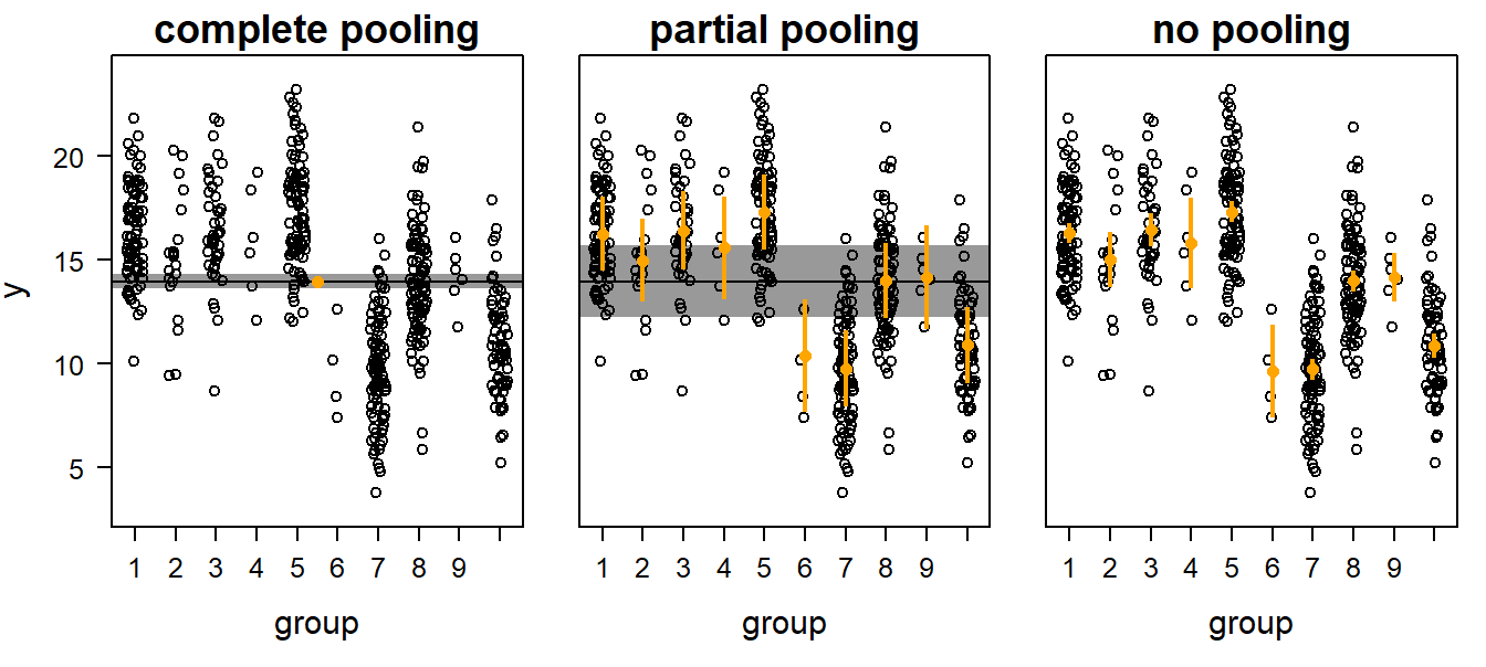
Figure 13.1: Three possibilities to obtain group and/or population means for grouped data: complete pooling, partial pooling, and no pooling. Open symbols = data, orange dots with vertical bars = group means with 95% uncertainty intervals, horizontal black line with shaded interval = population mean with 95% uncertainty interval.
What is the advantage of analyses using partial pooling (i.e., mixed, hierarchical, or multilevel modelling) compared to the complete or no pooling analyses? Complete pooling ignores the grouping structure of the data. As a result, the uncertainty interval of the population mean may be too narrow. We are too confident of the result because we assume that all observations are independent when they are not. This is a typical case of pseudoreplication. On the other hand, the no pooling method (which is equivalent to treating the factor as fixed) has the danger of overestimation of the among-group variance because the group means are estimated independently of each other. The danger of overestimating the among-group variance is particularly large when sample sizes per group are low and within-group variance large. In contrast, the partial pooling method assumes that the group means are a random sample from a common distribution. Therefore, information is exchanged between groups. Estimated means for groups with low sample sizes, large variances, and means far away from the population mean are shrunk towards the population mean. Thus, group means that are estimated with a lot of imprecision (because of low sample size and high variance) are shrunk towards the population mean. How strongly they are shrunk depends on the precision of the estimates for the group specific means and the population mean.
An example will help make this clear. Imagine that we measured 60 nestling birds from 10 nests (6 nestlings per nest) and found that the average nestling mass at day 10 was around 20 g with an among-nest standard deviation of 2 g. Then, we measure only one nestling from one additional nest (from the same population) whose mass was 12 g. What do we know about the average mass of this new nest? The mean of the measurements for this nest is 12 g, but with n = 1 uncertainty is high. Because we know that the average mass of the other nests was 20 g, and because the new nest belonged to the same population, a value higher than 12 g is a better estimate for an average nestling mass of the new nest than the 12 g measurement of one single nestling, which could, by chance, have been an exceptionally light individual. This is the shrinkage that partial pooling allows in a mixed model. Because of this shrinkage, the estimates for group means from a mixed model are sometimes called shrinkage estimators. A consequence of the shrinkage is that the residuals are positively correlated with the fitted values.
To summarize, mixed models are used to appropriately estimate among-group variance, and to account for non-independency among data points.
13.2 Fitting a normal linear mixed model in R
13.2.1 Background
To introduce the linear mixed model, we use repeated hormone measures at nestling barn owls Tyto alba. The cortbowl data set contains stress hormone data (corticosterone, variable “totCort”) of nestling barn owls which were either treated with a corticosterone implant, or with a placebo-implant as the control group. The aim of the study was to quantify the corticosterone increase due to the corticosterone implant (Almasi et al. 2009). In each brood, one or two nestlings were implanted with a corticosterone implant and one or two nestlings with a placebo implant (variable ‘Implant’). Blood samples were taken just before implantation, and at days 2 and 20 after implantation.
data(cortbowl)
dat <- cortbowl
dat$days <- factor(dat$days, levels=c("before", "2", "20"))
str(dat)  # the data was sampled in 2004,2005, and 2005 by the Swiss Ornithologicla Institute
## 'data.frame': 287 obs. of 6 variables:
## $ Brood : Factor w/ 54 levels "231","232","233",..: 7 7 7 7 8 8 9 9 10 10 ...
## $ Ring : Factor w/ 151 levels "898054","898055",..: 44 45 45 46 31 32 9 9 18 19 ...
## $ Implant: Factor w/ 2 levels "C","P": 2 2 2 1 2 1 1 1 2 1 ...
## $ Age : int 49 29 47 25 57 28 35 53 35 31 ...
## $ days : Factor w/ 3 levels "before","2","20": 3 2 3 2 3 1 2 3 2 2 ...
## $ totCort: num 5.76 8.42 8.05 25.74 8.04 ...In total, there are 287 measurements of 151 individuals (variable ‘Ring’) of 54 broods. Because the measurements from the same individual are non-independent, we use a mixed model to analyze these data. Two additional arguments for a mixed model are: a) The mixed model allows prediction of corticosterone levels for an ‘average’ individual, whereas the fixed effect model allows prediction of corticosterone levels only for each of the 151 individuals that were sampled. And b) fewer parameters are needed. If we include individual as a fixed factor, we would use 150 parameters, while the random factor needs a much lower number of parameters: we have one classical parameter, the among-individual variance; overall, the random factor increases model complexity by more than 1 parameter - by how many depends on the data, but it is usually much less than what is needed for a fixed factor with the same number of levels.
We first create a raw-data plot to show the development for each individual, separately for owls receiving corticosterone versus owls receiving a placebo (Figure 13.2).
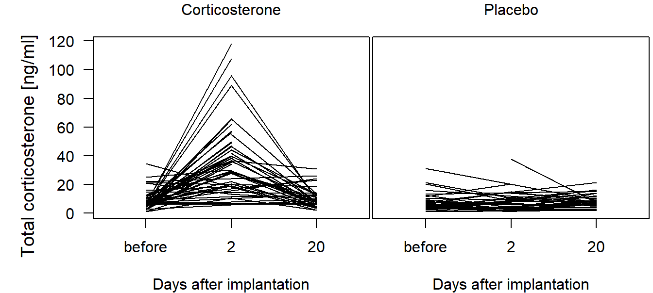
Figure 13.2: Total corticosterone before and at day 2 and 20 after implantation of a corticosterone or a placebo implant. Lines connect measurements of the same individual.
We fit a normal linear model with “Ring” (the individual) as a random factor, and “Implant” and “days”, including their interaction, as fixed effects. Note that both “Implant” and “days” are defined as factors, thus R creates indicator variables for all levels except the reference level. Later, we will also include “Brood” as a grouping level (i.e. random factor); for now, we ignore this level and start with a simpler (less perfect) model for illustrative purposes. The model can be written as follows:
\[ \begin{aligned} &\hat{y_i} = \beta_0 + b_{Ring_i} + \beta_1 I(days=2) + \beta_2 I(days=20) + \beta_3 I(Implant=P) \\ &\quad + \beta_4 I(days=2) I(Implant=P) + \beta_5 I(days=20) I(Implant=P) \\ &b_{Ring} \sim normal(0, \sigma_b) \\ &y_i \sim normal(\hat{y_i}, \sigma) \end{aligned} \]
The first part relates the fitted value of an observation (\(\hat{y_i}\), i.e. the expected value of the outcome variable) to the linear predictor. This linear predictor consists of the intercept \(\beta_0\) and five dummy variables for the factor levels (including the interaction) with their \(\beta\)-parameters (\(\beta_1\) to \(\beta_5\)), as we have seen it already for the simple linear model in Chapter 11.3.1. The new component of the linear predictor is the \(b_{Ring_i}\), which is an estimate per group: the deviation of each group from the overall mean. Adding these deviations to the intercept yields the group mean (assuming the baseline level for each factor, but using another level would just shift all the means by the same amount), using partial pooling as described above (= shrinkage estimator).
Several different functions to fit a mixed model have been written in R: lme, gls, gee have been the first ones. Then, lmer followed, and now, stan_lmer and brm allow to fit a large variety of hierarchical models (see also 11.1.2.4). We here start with using lmer from the package lme4, because it is kind of a basic function also for stan_lmer and brm. Further, sim can only work with lmer-objects but not the others. To work with lmer, we usually load the package arm which contains the function sim and also automatically loads the package lme4.
13.2.2 Fitting a normal linear mixed model using lmer, then use sim
The function lmer is used similarly to the function lm. The only difference is that the random factors are added to the model formula within parentheses, e.g. + (1|Ring). The “1” stands for the intercept and the “|” means “grouped by”. + (1|Ring), therefore, adds the random deviations for each individual (the \(b_{Ring_i}\) in the model formula above) from the overall mean.
To fit the model to our example data, we log-transformed the corticosterone values (i.e. the outcome variable) to achieve normally distributed residuals. After having fitted the model, in real life, we always first inspect the residuals before we look at the model output. Here, we skip this point to explain how the model is constructed right after having shown the model code. But we will come back to the residual analyses.
## Linear mixed model fit by REML ['lmerMod']
## Formula: log(totCort) ~ Implant + days + Implant:days + (1 | Ring)
##    Data: dat
## REML criterion at convergence: 611.9053
## Random effects:
##  Groups   Name        Std.Dev.
##  Ring     (Intercept) 0.3384
##  Residual             0.6134
## Number of obs: 287, groups:  Ring, 151
## Fixed Effects:
##     (Intercept)         ImplantP            days2           days20
##         1.91446         -0.08523          1.65307          0.26278
##  ImplantP:days2  ImplantP:days20
##        -1.71999         -0.09514
The output of the lmer-object tells us that the model was fitted using the REML-method, which is the restricted maximum likelihood method. The “REML criterion” is the statistic describing the model fit for a model fitted by REML. Then follows the more interesting part: the parameter estimates. These are grouped into a random effects and fixed effects section. The random effects section gives the estimates for the among-individual standard deviation of the intercept
Neither the model output shown above nor the summary function (not shown) give any information about the proportion of variance explained by the model such as an \(R^2\). The reason is that it is not straightforward to obtain a measure of model fit in a mixed model, and different definitions of \(R^2\) exist (Nakagawa and Schielzeth 2013). Check out the function r.squaredGLMM from package MuMIn to get pseudo-\(R^2\) for mixed models.
The function fixef extracts the estimates for the fixed effects, the function ranef extracts the estimates for the random deviations from the population intercept for each individual. The ranef-object is a list with one element for each random factor in the model. We can extract the random effects for each ring using the $Ring notation.
##     (Intercept)        ImplantP           days2          days20  ImplantP:days2
##           1.914          -0.085           1.653           0.263          -1.720
## ImplantP:days20
## -0.095## (Intercept)
## 898054 0.24884979
## 898055 0.11845863
## 898057 -0.10788277
## 898058 0.06998959
## 898059 -0.08086498
## 898061 -0.08396839As done with a normal linear model in Chapter 11, we also use the function sim to draw (e.g.) 2000 random values from the joint posterior distribution of the model parameters; that is, we draw 2000 values for each parameter while taking the correlation between the parameters into account.
## Formal class 'sim.merMod' [package "arm"] with 3 slots
##   ..@ fixef: num [1:2000, 1:6] 2.03 1.87 1.96 2.07 1.86 ...
##   .. ..- attr(*, "dimnames")=List of 2
##   .. .. ..$ : NULL
##   .. .. ..$ : chr [1:6] "(Intercept)" "ImplantP" "days2" "days20" ...
##   ..@ ranef:List of 1
##   .. ..$ Ring: num [1:2000, 1:151, 1] 0.7891 -0.076 0.1704 -0.0165 0.0768 ...
##   .. .. ..- attr(*, "dimnames")=List of 3
##   .. .. .. ..$ : NULL
##   .. .. .. ..$ : chr [1:151] "898054" "898055" "898057" "898058" ...
##   .. .. .. ..$ : chr "(Intercept)"
##   ..@ sigma: num [1:2000] 0.646 0.602 0.585 0.626 0.61 ...
The object produced by the sim function when applied to a mer object (= object produced by the functions lmer or glmer) contains three slots (remember that slots are addressed using the @ sign in R). The slot “fixef” is a matrix with as many columns as there are parameters in the fixed part of the model. The number of rows corresponds to the number of simulations (we have saved this number in the object “nsim”). The slot “ranef” is a list that contains one element for each random factor. In the our example, there is only one random factor (“Ring”). Therefore, the list contains only one element. The slot “sigma” contains the draws from the posterior distribution of the residual standard deviation.
Each element of the ranef slot is a three-dimensional array where the first dimension represents the number of simulations (2000 in our case), the second dimension is the number of groups (factor levels; here this is the number of individuals), and the third dimension corresponds to the number of parameters that are grouped by the specific factor. In the our example, we have included only a random intercept in the model. Therefore, this dimension has a length of one. Later, we will fit models with more parameters per random effect.
From the draws (i.e. draws from the joint posterior distribution), the 2.5% and 97.5% quantiles can be used as a 95% compatibility interval:
##       (Intercept) ImplantP days2 days20 ImplantP:days2 ImplantP:days20
## 2.5%        1.741   -0.347 1.409  0.007         -2.072          -0.448
## 50%         1.913   -0.090 1.657  0.263         -1.712          -0.089
## 97.5%       2.082    0.175 1.894  0.498         -1.362           0.269
We come back to the interpretation of these values in the chapter below on how to present the results from this lmer-model. First, we provide some extra information on REML, then we check some model assumptions. After that, we fit the same model using rstanarm and brms. Then, we suggest how the present the results for each of our three model fitting approaches: lmer + sim, rstanarm (function stan_lmer), and brms (function brm).
13.2.2.1 Restricted maximum likelihood estimation (REML)
For a mixed model the restricted maximum likelihood method is used by default instead of the maximum likelihood (ML) method (see Chapter 9.3). The reason is that the ML-method underestimates the variance parameters because this method assumes that the fixed parameters are known without uncertainty when estimating the variance parameters. However, the estimates of the fixed effects have uncertainty. The REML method uses a mathematical trick to make the estimates for the variance parameters independent of the estimates for the fixed effects. We recommend reading the very understandable description of the REML method in Zuur et al. (2009). For our purposes, the relevant difference between the two methods is that the ML-estimates are unbiased for the fixed effects but biased for the random effects, whereas the REML-estimates are biased for the fixed effects and unbiased for the random effects. However, when sample size is large compared to the number of model parameters, the differences between the ML- and REML-estimates become negligible. As a guideline, use REML if the interest is in the random effects (variance parameters), and ML if the interest is in the fixed effects. The estimation method can be chosen by setting the argument ‘REML’ to ‘FALSE’ (default is ‘TRUE’).
mod <- lmer(log(totCort) ~ Implant + days + Implant:days + (1|Ring),
            data=dat, REML=FALSE)  # using ML
When we fit the model by stan_lmer from the rstanarm-package or brm from the brms-package, i.e., using the Bayes theorem instead of ML or REML, we do not have to care about this choice (of course!). The result from a Bayesian analyses is unbiased for all parameters (at least from a mathematical point of view - also parameters from a Bayesian model can be biased if the model violates assumptions or is confounded).
13.2.2.2 Assessing model assumptions for the lmer fit
As with a simple linear model, the assumptions are carefully checked before inference is drawn from a mixed model. The assumptions are, as explained in Chapter 12, that the residuals are independent and identically distributed (iid). In principle, the same methods described in Chapter 12 are used to assess violation of model assumptions in mixed models. However, the function plot does not produce the standard diagnostic residual plots from an lmer object. Therefore, these plots have to be coded by hand.
In the first plot of Figure 13.3 we see that the residuals scatter around zero with a few exceptions in the lower left part of the panel. A positive correlation between the residuals and the fitted values (not present in the example data) would not bother us statistically in the case of a mixed model, but it indicates strong shrinkage and may have biological meaning.
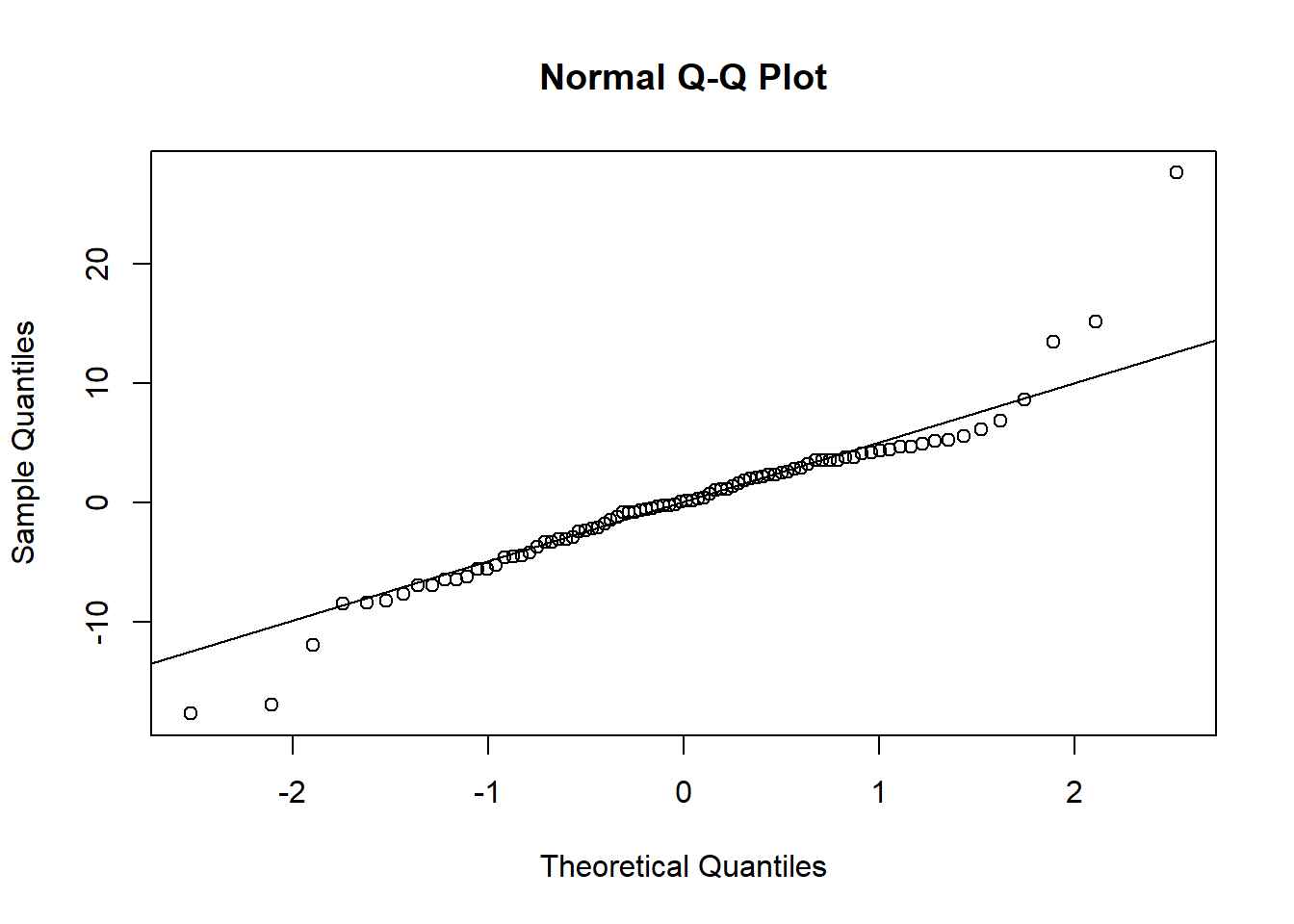
The few small measurements that do not fit well to the model are also recognizable in the QQ plot of the residuals (a banana-like deviation from the straight line at the left edge of the data) and when plotting the square root of the absolute values of the residuals against the fitted values (second and third plots in Figure 13.3). Because the number of such cases is low and all other observations seem to fulfill the model assumptions well, we accept the slight lack of fit. But we are aware of the fact that model predictions for small corticosterone levels are unreliable.
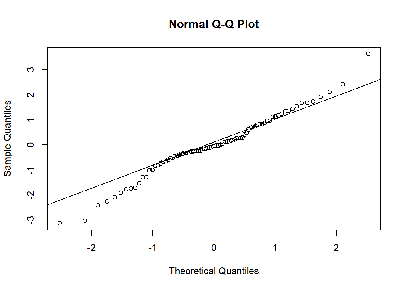
In addition to the checks presented in Chapter 12, the assumption that the random effects, that is the values of \(b_{Ring}\), are normally distributed, needs to be checked. We do this using a QQ plot (fourth plot in Figure 13.3). Note that we need to extract the \(b_{Ring}\) using “[,1]” because the ranef object is two-dimensional.
par(mfrow=c(2,2))
scatter.smooth(fitted(mod),resid(mod)); abline(h=0, lty=2)
title("Tukey-Anscombe Plot") # residuals vs. fitted

qqnorm(resid(mod), main="normal QQ-plot, residuals") # qq of residuals
qqline(resid(mod))
scatter.smooth(fitted(mod), sqrt(abs(resid(mod)))) # res. var vs. fitted

qqnorm(ranef(mod)$Ring[,1], main="normal QQ-plot, random effects")
qqline(ranef(mod)$Ring[,1]) # qq of random effects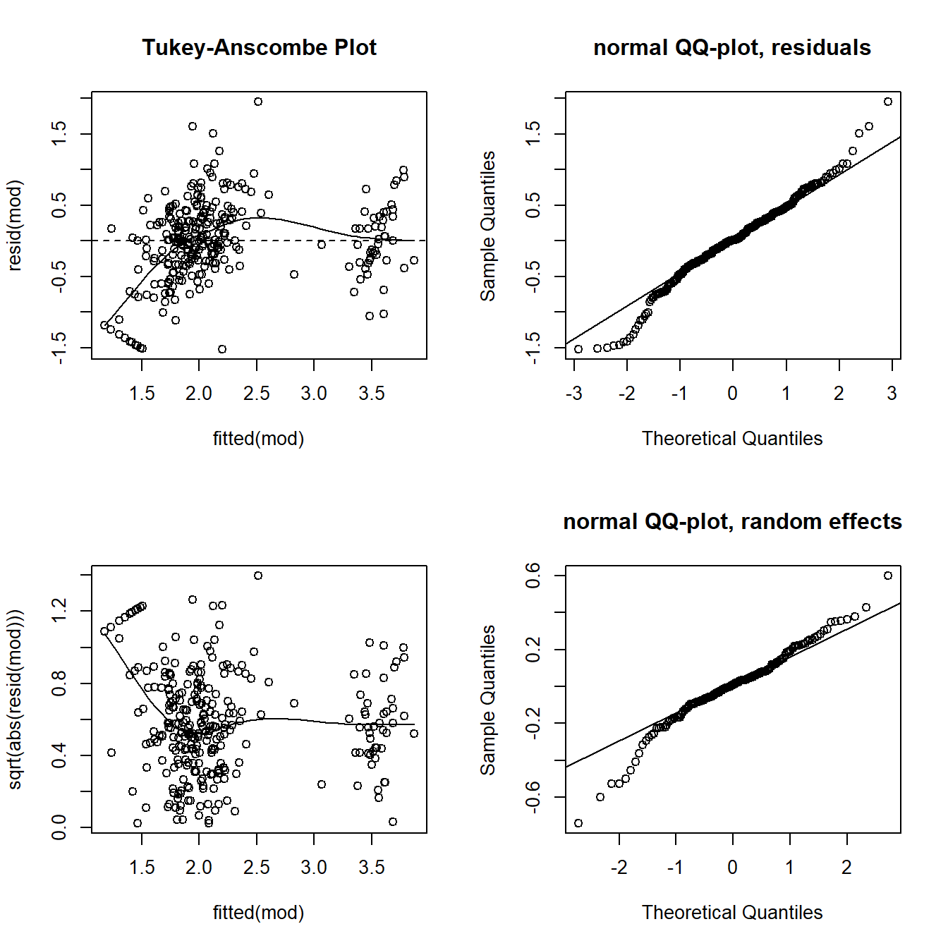
Figure 13.3: Diagnostic residual and random effect plots to assess model assumptions of the corticosterone model. Upper left: residuals versus fitted values. Upper right: Normal QQ plot of the residuals. Lower left: square-root of the absolute values of the residuals versus fitted values. Lower right: Normal QQ plot of the random effects.
We do not see a serious deviation in the distribution of the random effects from the normal distribution. Remember from the chapter on partial pooling and shrinkage (Chapter 13.1.2) that a positive correlation between fitted values and residuals often shows up in mixed models - this is due to shrinkage and not a violation of model assumptions. In our example, we don’t see such an effect, hence shrinkage does not seem to be very strong.
13.2.3 Fitting a normal linear model using rstanarm
Above, we fitted a linear mixed effects model using lmer. Here, we fit the same model using the package rstanarm. For that, we apply the function stan_lmer; the model formula remains unchanged, but we don’t need to worry about the REML-argument (Chapter 13.2.2.1):
# lmer-call from above for comparison:
# mod <-             lmer(log(totCort) ~ Implant + days + Implant:days + (1|Ring),
#                         data=dat, REML=TRUE)
mod.rstanarm <- stan_lmer(log(totCort) ~ Implant + days + Implant:days + (1|Ring),
                          data=dat, refresh=0)
stan_lmer is “fully Bayesian” (while lmer is not Bayesian, and lmer + sim returns Bayesian draws from the posterior not in a fully Bayesian way, i.e. it assumes flat priors and this cannot be changed). Therefore, it is possible to use custom priors if needed. By default, rstanarm uses weakly informative priors which helps model convergence. You can get the priors used applying the function prior_summary on the model object, i.e. “mod.rstanarm” in our example.
You can set additional arguments (that are not available / needed in lmer) such as weights and settings for the MCMC sampling (see Chapter 11.1.2.4).
Checking model assumptions will be addressed together with the model fitted using brm, done next.
13.2.4 Fitting a normal linear model using brm
As with rstanarm, fitting the linear mixed effects model with brm is straightforward. Because compiling the model takes a little time, we here save the compiled model (as we did with the analogous normal linear model), but this is optional.
 # mod.lmm.brm.compiled <- brm(log(totCort) ~ Implant + days + Implant:days + (1|Ring),
 #                         data=dat, chains=0)
 # save(mod.lmm.brm.compiled,file="RData/mod.lmm.brm.compiled.RData")
load("RData/mod.lmm.brm.compiled.RData")
mod.brm <- update(mod.lmm.brm.compiled, recompile = FALSE, seed=123, refresh=0)
The priors used can be accessed using prior_summary(mod.brm). If needed, you can change the priors using set_prior. You can adjust the MCMC settings by different arguments of brm, e.g. iter, warmup. In brm, you can also add other model components such as autocorrelation, weighting and more. If you get warnings, check Chapter 18.
13.2.4.1 Assessing model assumptions for the rstanarm and brm fit
We can and should do similar model checking as we can do with an object from lmer, see the chapter above. We can use the function fitted and resid as above, but there is a difference for the brm-object: these functions don’t only return a point estimate for the fitted value or the residual, but also, for each of them, a standard error and a 2.5% and 97.5% quantile (i.e. the 95% compatibility interval for each fitted value / for each residual). Hence, for the plots, we generally have to specify that we only want the point estimate, labelled “Estimate”:
t.res <- resid(mod.brm)[,"Estimate"] # because we need that several times, we store it in a temporary object
scatter.smooth(fitted(mod.brm)[,"Estimate"], t.res); abline(h=0, lty=2)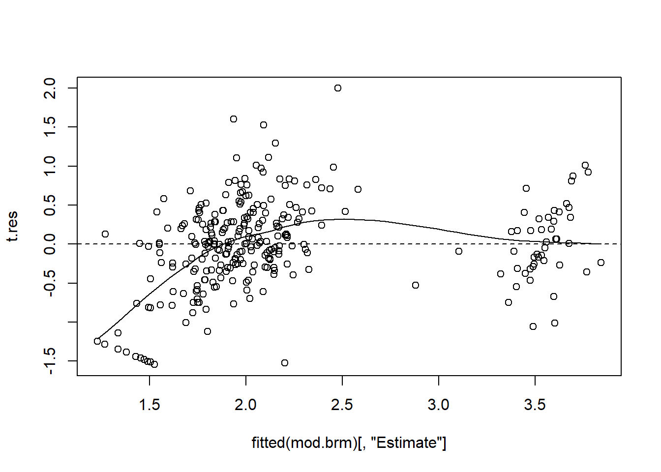
Remember again: if there is a positive correlation in this plot, it is likely due to shrinkage (Chapter 13.1.2) and not a violation of model assumptions.
You can use “t.res” to make the other residual plots such as residuals vs. each predictor (checks whether the assumption of a linear relationship is reasonable), residual QQ plot, or, if needed, plots to check for temporal or spatial autocorrelation.
For the residual plots suggested above (for the lmer-fitted model) regarding random term check out str(ranef(mod.rstanarm)) and str(ranef(mod.brm)): from these you see that the random intercepts for the “Ring” random factor can be accessed using ranef(mod.rstanarm)$Ring[,"(Intercept)"] and ranef(mod.brm)$Ring[,"Estimate",], respectively (the 2nd dimension for the brm-case has names “Estimate”, “Est.Error”, “Q2.5”, “Q97.5” - for here, we only need the “Estimate”).
One of the best ways to check several model assumptions (linearity, data distribution) is posterior predictive model checking, which is explained in Chapter 16 in the context of a generalize linear mixed model. And the really great thing about using rstanarm or brm is that we can very easily do posterior predictive model checking. The principal is very simple: we use the model to generate new data (this means that we use the observed predictor values and generate new outcome variable values, one for each data row). If our model is a good model, the generated data (i.e. new log-totCourt values in our case) should look similar to the real data (i.e. the real log-totCourt values). We can also do that based on the object generated by sim (i.e. approach lmer + sim), but it takes more coding. With an rstanarm-object, this is the code:
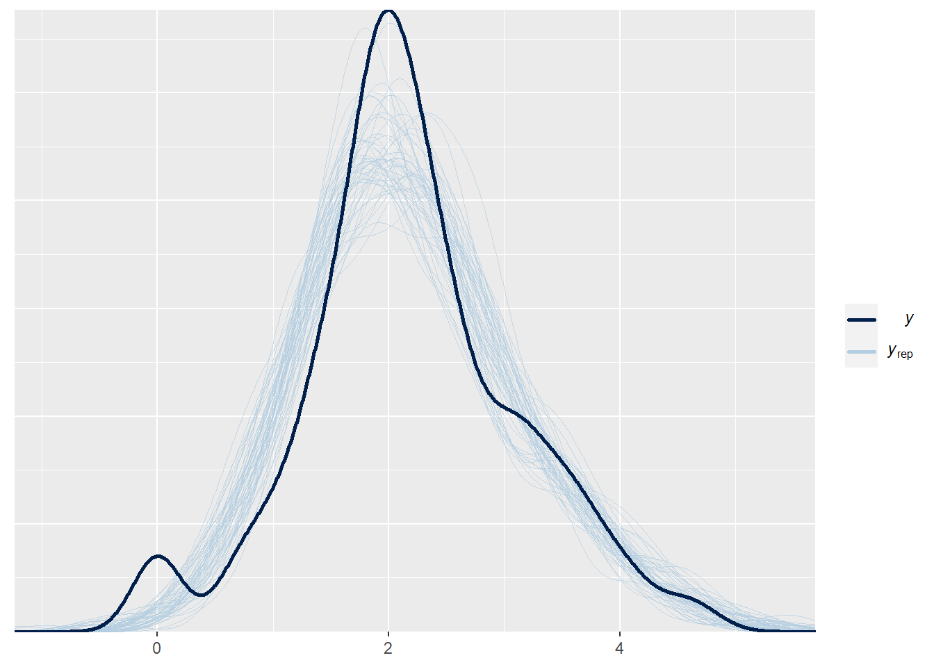
We see in dark blue the distribution of the observed log-totCort values, and in lightblue the distribution from many model-generated log-totCort values (using the predictor values of the original data). We see an overall good concordance between the real data and the model-generated data. We see a little deviation at very small log-totCort values, where the real data has a slight local peak. We can check in the data why there are these small values. If they are not errors, and if we are absolutely interested in modelling this aspect of the data, our model is not a good model - it does not capture the small peak of small values. But, more likely, what happens there is not very important for our biological question, and we can be happy with the model.
We look at other checks we can do based on data generated from the model, i.e. by posterior predictive model checking, in @Chapter(postpredmodcheck).
13.3 Presenting the results
13.3.1 Presenting the results: from sim
Above, we have used the function sim to draw 2000 random values from the joint posterior distribution of the model parameters. We generated the point estimates and 95% compatibility intervals for each parameter using:
##       (Intercept) ImplantP days2 days20 ImplantP:days2 ImplantP:days20
## 2.5%        1.741   -0.347 1.409  0.007         -2.072          -0.448
## 50%         1.913   -0.090 1.657  0.263         -1.712          -0.089
## 97.5%       2.082    0.175 1.894  0.498         -1.362           0.269
Some effort is needed to interpret models with interactions (independent of whether it is a mixed model or not). We see that in the corticosterone-treated nestlings, the logarithm of the corticosterone measure increases from before implantation to day 2 by 1.7 (95% compatiblity interval CI: 1.4-1.9), which is quite substantial. To get this increase for the placebo-treated individuals, we have to add the interaction parameter, thus the increase in placebo nestlings is 1.7-1.7 = 0. The interaction parameter, -1.7 (95% CI: -2.1 to -1.4), measures the difference between placebo and corticosterone nestlings in their response to the treatment; it is, therefore, an important result.
To better see what really happens, we plot the fitted values with its CI and (optionally but often with additional benefit) the observations in one plot. To this end, we first prepare a new data frame that contains a row for each factor level (“Implant” and “days”). Then, the fitted value for each of the factor-level combinations is calculated 2000 times (once for each set of model parameters from the simulated posterior distribution) to obtain 2000 simulated values from the posterior distribution of the fitted values. The 2.5% and 97.5% quantiles of these fitted values are used as lower and upper bounds of the 95% compatibility interval.
newdat <- expand.grid(Implant=factor(c("C","P"),levels=levels(dat$Implant)),
                      days=factor(c("before",2,20),levels=levels(dat$days)))
Xmat <- model.matrix(~ Implant + days + Implant:days, data=newdat)
fitmat <- matrix(ncol=nsim, nrow=nrow(newdat))
for(i in 1:nsim) fitmat[,i] <- Xmat %*% bsim@fixef[i,] # fitted values
newdat$lower <- apply(fitmat, 1, quantile, prob=0.025)
newdat$upper <- apply(fitmat, 1, quantile, prob=0.975)
newdat$fit <- Xmat %*% fixef(mod)
The fitted values given in Figure 13.4, together with their uncertainty measures (compatibility intervals), take into account that we had repeated measures for each individual.
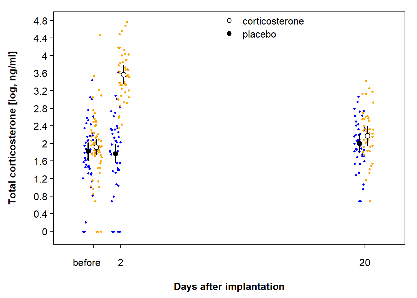
Figure 13.4: Predicted total corticosterone values with 95% CI of placebo-implanted nestlings (closed symbol) and corticosterone-implanted nestlings (open symbol) in relation to days after implantation. Blue dots are raw data of placebo-implanted nestlings, and orange dots are raw data of corticosterone-implanted nestlings.
13.3.2 Presenting the results: from rstanarm
We present in more detail the advantages and differences of extracting the parameter estimates and their 95% compatibility intervals in the normal linear model chapter (11). From the rstanarm model, we still need the “newdat” object created above, but we can then use posterior_epred, i.e. we don’t have to do the model matrix multiplication done above.
There is one additional thing we have do do in the case of a mixed model: posterior_epred predicts taking all random effects into account. For an effectplot, we typically want to show the population estimate, not a separate estimate for random levels. Hence, we have to set the argument re.form=NA. If you forget, there will be an error, because the newdat does not contain the random factor.
  # newdat generated as above. Remember to ascertain that the factor level ordering in
  # newdat is the same as in dat - else you will mix up the estimates among factor levels,
  # if levels are not alphanumeric!
newdat.rstanarm <- expand.grid(Implant=factor(c("C","P"),levels=levels(dat$Implant)),
                               days=factor(c("before",2,20),levels=levels(dat$days)))
fitmat.rstanarm <- posterior_epred(mod.rstanarm, newdata=newdat, re.form=NA)
From this, you proceed as with the “fitmat” from above.
13.3.3 Presenting the results: from brms
We can use the function conditional_effects to make effectplots from a brm-fitted model. There is no need to create “newdat” by hand, as done above. contional_effects also makes a plot, but generally it may be better to store the values in a “newdat” and use that to make your custom plot. Since we have an interaction in the model, it makes no sense to only plot for “Implant” or only for “days”. Hence, we set effects=c("Implant:days) to get estimates (and 95% compatibility intevals) for all combinations of the two factors.
And: other than with posterior_epred, the default of conditional_effects is to not consider random effects (the default for the argument, here called re_formula, is NA).
Now, again, use newdat.brm to make the plot as you please.
posterior_epred makes generating effectplots easier, conditional_effects makes it very easy. For both functions, this is especially true when you want to predict for random factors, and very especially if you have random slopes (next chapter) - then is becomes brain gym if you want to do it using lmer + sim (or glmer + sim). We do some of that brain gym in the next chapter, but before it starts, we remember you that using rstanarm or brm makes simplifies this considerably.
13.4 Random intercept and slope
In the preceding model, only the intercept \(\beta_0\) was modeled per individual (the model allowed for between-individual variance in \(\beta_0\)). But a random effect does not need to be restricted to the intercept. Any parameter can be modeled, if the data allow. For example, in the previous model we cannot include an individual-specific difference between corticosterone and placebo treatment because each individual obtained only one treatment. Therefore, the data do not contain information about between-individual differences in the treatment effect, and it does not make sense to include such a structure in the model. In another study on barn owls, we were interested in the effect of corticosterone on growth rate. Here, we measured wing length (as a proxy for size) at different ages of individuals that had been treated either with corticosterone or with a placebo implant. We used the slope of the regression line for wing length on age as a growth rate measure, and we were interested in the difference in this slope between corticosterone- and placebo-implanted individuals. We expected that growth rate differed between individuals due to between-individual differences in body condition and also because the age at which the implant was implanted differed between the individuals because barn owl nestlings hatch asynchronously (the implantation was done on the same day for all the nestlings in a nest). Therefore, we modeled the slope of the regression line for each individual. Otherwise, our confidence in the (population) slope parameter would be too high (the compatibility intervals would be too narrow). This is because individual-specific slopes in the data produce a kind of pseudoreplication when equal slopes between individuals are assumed in the model (Schielzeth and Forstmeier (2009)). The data for the growth rate study are in the wingbowl data set. In total, we have 209 measurements of 86 individuals (variable “Ring”) from 24 broods. In the model, we include “age” (as a continuous covariate), “implant” (as a fixed effect), and their interaction in the fixed part; and “ring” (= id of individual) is included as a random effect. We model both the intercept and the slope for the covariate “age” dependent on “ring.” We use this notation with \(b_{Ring}\) being an individual-specific deviation from the population mean parameter value, but we add a second numerical subscript, \(b_{1,Ring}\), to indicate the random intercept and \(b_{2,Ring}\) for the random slope. The two random parameters are assumed to follow a multivariate normal distribution (MVNorm); that is, they are both normally distributed and are assumed to be correlated and this correlation is estimated. Hence, the formula for the random intercept and random slope model is:
\[ \begin{aligned} &\hat{y_i} =\beta_0 + b_{1,Ring_i} + (\beta_1 + b_{2,Ring_i}) age_i + \beta_2 I(Implant=P)+\beta_3 age_i I(Implant=P) \\ &y_i \sim normal(\hat{y_i}, \sigma^2) \\ &\boldsymbol{b}_{1:2,Ring} \sim MVnormal(\boldsymbol{0,\Sigma}) \end{aligned} \]
The vector \(\boldsymbol{b}_{1:2,Ring}\) contains the two parameters \(b_{1,Ring}\) and \(b_{2,Ring}\). The matrix \(\boldsymbol{\Sigma}\) contains the variances of and the covariances between the intercept and the slope. The notation (Age|Ring) means that both the intercept and the Age-effect are grouped by Ring. We find it advisable to center and scale covariates, especially for mixed models with some complexity because non-centered covariates lead to a stronger correlation between the estimated parameters, which may cause nonconvergence of the fitting algorithm. Hence, we center and scale the variable “Age”:
data(wingbowl)
dat <- wingbowl
dat$Age.z <- scale(dat$Age)
mod <- lmer(Wing ~ Age.z + Implant + Age.z:Implant + (Age.z|Ring),
            data=dat, REML=FALSE)
mod
## Linear mixed model fit by maximum likelihood ['lmerMod']
## Formula: Wing ~ Age.z + Implant + Age.z:Implant + (Age.z | Ring)
## Data: dat
## AIC BIC logLik deviance df.resid
## 1280.4391 1307.1778 -632.2195 1264.4391 201
## Random effects:
## Groups Name Std.Dev. Corr
## Ring (Intercept) 6.394
## Age.z 1.898 -0.12
## Residual 2.542
## Number of obs: 209, groups: Ring, 86
## Fixed Effects:
## (Intercept) Age.z ImplantP Age.z:ImplantP
## 155.442 24.954 4.554 2.185The estimate of the between-nestling standard deviation for the intercept is 6.4 and for the age-effect (slope), this value is 1.9. We see that there is a negative correlation between the intercept and the slope (-0.12). This is not unusual, and it would be even stronger with noncentered predictors: this means we can find different regression lines that fit the data similarly well when we increase the intercept and simultaneously decrease the slope.
We can use the diagnostic residual plots as described in Chapter 12, and the R code of the previous section, to produce a QQ plot of the random effects. Because two parameters were modeled per individual, we have to produce two different QQ plots to assess whether the random effects are normally distributed. The different parameters for each random effect are extracted from the ranef object using the squared brackets because the random effects are given as a matrix containing one row per individual and one column per parameter (here: intercept and age-effect).
The diagnostic residual plots did not indicate strong violation of the model assumptions; therefore, we can start drawing inferences from the model. Our question was how strongly does corticosterone affect growth rate? From the model output we see that individuals with a placebo implant grow 2.2 mm more per standard deviation of age, that is, 2.2/sd(dat$Age) = 0.4 mm per day compared to the individuals with a corticosterone implant. We can get the 95% CI of the parameter estimates using sim.
##       (Intercept)    Age.z ImplantP Age.z:ImplantP
## 2.5%     153.3527 24.01732 1.716015       0.851704
## 97.5%    157.4189 25.89176 7.474940       3.549412
The CI for the interaction effect of 0.4 mm, on the original Age-scale, is:
##      2.5%     97.5%
## 0.1603468 0.6682333
Thus, given the data and the model, we are 95% sure that the wings of placebo nestlings grow between 0.16 mm and 0.66 mm faster per day than the wings of corticosterone nestlings. To be better able to assess the biological relevance of this effect, we may want to plot the two regression lines (averaged over the individuals) as well as the individual-specific regression lines (13.5). To do so, we calculate the fitted values for each age and implant combination 2000 times, each with a different set of model parameters from their posterior distribution.
newdat <- expand.grid(Age=seq(23, 45, length=100),
                      Implant=levels(dat$Implant))
newdat$Age.z <- (newdat$Age - mean(dat$Age))/sd(dat$Age)
Xmat <- model.matrix(~Age.z + Implant + Age.z:Implant, data=newdat)
fitmat <- matrix(ncol=nsim, nrow=nrow(newdat))
for(i in 1:nsim) fitmat[,i] <- Xmat %*% bsim@fixef[i,]
newdat$lower <- apply(fitmat, 1, quantile, prob=0.025)
newdat$upper <- apply(fitmat, 1, quantile, prob=0.975)
Now follows, as warned above, some brain gym to get the effect plot including the random factor. As also stated above, it would be easier to include the random effect levels in “newdat” and then use posterior_epred or, with no need for a newdat, conditional_effects, but for these, you need to fit the model with rstanarm or brms (conditional_effects only works with a brms-object).
We do not extract the mean of the posterior distribution of the fitted values because we use the ML estimates for drawing the mean regression lines. These estimates are not subject to simulation error. Note that we use Age.z on the x-axis, but we label the x-axis with back-transformed values so that we are able to use the abline function to draw the regression lines directly from the model parameters.
To draw the individual-specific regression lines, we add the individual-specific deviations from the intercept and the slope, respectively, to the population intercept and slope.We do this in a separate plot so as not to overload the figure.
par(mfrow=c(1,2), mar=c(5,1,1,0.1), oma=c(0,4,0,0))
plot(dat$Age.z, dat$Wing, pch=1, cex=0.8, las=1,xlab="Age (days)",
     col=c("orange", "blue")[as.numeric(dat$Implant)],ylab=NA, xaxt="n")
at.x_orig <- seq(25,45,by=5) # values on the x-axis, original scale
at.x <- (at.x_orig-mean(dat$Age))/sd(dat$Age) # transformed scale
axis(1, at=at.x, labels=at.x_orig) # original values at transformed
mtext("Wing length (mm)", side=2, outer=TRUE, line=2, cex=1.2, adj=0.6)
abline(fixef(mod)[1], fixef(mod)[2], col="orange", lwd=2) # for C
abline(fixef(mod)[1]+fixef(mod)[3], fixef(mod)[2]+fixef(mod)[4], col="blue", lwd=2) # for P
# add transparent polygons to visualize the 95% CI
for(i in 1:2){
  index <- newdat$Implant==levels(newdat$Implant)[i]
  polygon(c(newdat$Age.z[index], rev(newdat$Age.z[index])),
          c(newdat$lower[index], rev(newdat$upper[index])),
          border=NA, col=c(rgb(1,0.65,0,0.5), rgb(0,0,1,0.5))[i])
}
legend(x=-1.5,y=100, c("corticosterone", "placebo"),pch=c(1,1),col=c("orange","blue"),
       bty="n",lwd=2,cex=1, pt.cex=1.2)

# individual-specific regression lines in a separate plot:
plot(dat$Age.z, dat$Wing, pch=1, cex=0.8, las=1, col=c("orange", "blue")[as.numeric(dat$Implant)],
     xlab="Age (days)", ylab=NA, yaxt="n", xaxt="n")
at.x_orig <- seq(25,45,by=5)
at.x <- (at.x_orig - mean(dat$Age))/sd(dat$Age)
axis(1, at=at.x, labels=at.x_orig)
indtreat <- tapply(dat$Implant, dat$Ring, function(x) as.character(x[1]))
for(i in 1:86){
  if(indtreat[i]=="C")
    abline(fixef(mod)[1]+ranef(mod)$Ring[i,1],
           fixef(mod)[2]+ranef(mod)$Ring[i,2],col="orange")
  else
    abline(fixef(mod)[1]+fixef(mod)[3]+ranef(mod)$Ring[i,1],
           fixef(mod)[2]+fixef(mod)[4]+ranef(mod)$Ring[i,2],col="blue")
}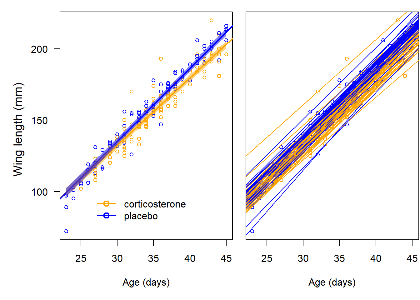
Figure 13.5: Left: Population regression lines (bold lines) with 95% compatibility intervals (semitransparent color) for the corticosterone (orange) and placebo (blue) treated barn owl nestlings. Right: Individual-specific regression lines. Circles are the raw data.
We see a discernible effect of corticosterone on growth rate such that the wing length of corticosterone-treated nestlings is, on average, around 1 cm smaller than in placebo-treated individuals at the end of the nestling phase.
13.5 Nested and crossed random effects
Random factors can be nested or crossed. Each level of a factor that is nested within another factor occurs only in one level of the other factor (Figure 13.6, left). For example, the factor “nestling” is nested in the factor “nest” because the same nestling cannot be in two nests. In contrast, when two factors are crossed, all possible combinations of the factor levels occur in the data set (Figure 13.6, right). For example, the factors “month” and “year” are crossed, because all months occur in every year.

Figure 13.6: Nested and crossed structures of two factors. In the left panel, each level of the factor "individual" only occurs in one level of the factor "nest". These are called nested effects. In the right panel, each level of the factor "species" occurs in all levels of the factor "field". Therefore, these factors are called crossed.
It is important to specify factors as nested and crossed random factors, because a falsely specified structure leads to indecipherable results. If unique level names are used (in contrast to starting with the number 1 in each group), the nested structure is defined in the data and there is no need to explicitly specify the nested design in the lmer (or glmer, see Chapter 15) function; if nestlings (or other levels nested in another factor) are not labeled uniquely (i.e., different nestlings from different nests have the same name), the nesting structure has to be specified in the model formula. The following is an example of a nested random effect and one of a crossed random effect.
In the two barn owl example data sets described earlier, the individuals were actually not independent because they were grouped in nests. Thus, we should have included nest as another random factor in the two models. Because each individual only appears in one nest, these two random factors are nested. There are two possible ways to specify nested random effects in the function lmer. The first is to add the factor nest (“Brood”) as a second random effect in the model formula. This only fits nested random effects if the nested structure is clear from the names of the factor levels, because the nested structure is not explicitly defined in the model formula; all nestlings must have a unique name, thereby, it becomes clear that each nestling belongs to only one nest (is nested within nest).
data(cortbowl)
dat <- cortbowl
mod <- lmer(log(totCort) ~ Implant + days + Implant:days
            + (1|Brood) + (1|Ring), data=dat, REML=FALSE)
mod
## Linear mixed model fit by maximum likelihood ['lmerMod']
## Formula: log(totCort) ~ Implant + days + Implant:days + (1 | Brood) +
## (1 | Ring)
## Data: dat
## AIC BIC logLik deviance df.resid
## 604.2934 637.2287 -293.1467 586.2934 278
## Random effects:
## Groups Name Std.Dev.
## Ring (Intercept) 0.1917
## Brood (Intercept) 0.2486
## Residual 0.6117
## Number of obs: 287, groups: Ring, 151; Brood, 54
## Fixed Effects:
## (Intercept) ImplantP days20
## 3.592 -1.796 -1.383
## daysbefore ImplantP:days20 ImplantP:daysbefore
## -1.639 1.617 1.693The second possibility is to define explicitly the nested structure in the model formula using the “F1/F2” notation (“F2 is nested in F1”).
mod <- lmer(log(totCort) ~ Implant + days + Implant:days
            + (1|Brood/Ring), data=dat, REML=FALSE)
summary(mod)$varcor
## Groups Name Std.Dev.
## Ring:Brood (Intercept) 0.19168
## Brood (Intercept) 0.24863
## Residual 0.61170These two models are the same, hence not all model output is repeated. The only difference is in the name of the individual random factor: it is called “Ring” in the first version, whereas in the second version it is called “Ring:Brood”, meaning “Ring nested in Brood”.
To specify crossed random effects, we can only use the first specification in the previous example. For example, in Ellenberg’s data (Chapter 11), six different grass species were grown in four different situations: two tanks in each of two years, and the two tanks contained different soil. This four-level factor has been called “gradient” by Hector et al. (2012). Four species were grown in all four gradients and two species were grown in only two of the gradients. Above-ground biomass was measured for 11 different water conditions within each species-gradient combination.
data(ellenberg)
ellenberg$gradient <- paste(ellenberg$Year, ellenberg$Soil)
table(ellenberg$Species, ellenberg$gradient)
##
## 1952 Loam 1952 Sand 1953 Loam 1953 Sand
## Ae 11 11 11 11
## Ap 11 11 11 11
## Be 11 11 11 11
## Dg 11 11 11 11
## Fp 11 11 0 0
## Pp 11 11 0 0We assume that the six grass species are a random sample from the family Poaceae (true grasses) and we may be interested in the general relationship between water condition (distance to ground water; using a linear and a quadratic term) and Poaceae biomass, as well as in species-specific reactions to water conditions. Therefore, we treat species as a random factor. We also include gradient as a random factor to correct for any between-gradient variance.
ellenberg$water.z <- as.numeric(scale(ellenberg$Water))
mod <- lmer(log(Yi.g) ~ water.z + I(water.z^2)
            + (water.z + I(water.z^2)|Species) + (1|gradient), data=ellenberg)
We did not find any suspicious pattern in the residuals and, therefore, plot the species-specific and the overall (for all Poaceae) relationship between water gradient and biomass in a figure. We see that the average biomass of Poaceae does not change with distance to ground water, but the different species react quite differently to the water condition (13.7).

Figure 13.7: Average biomass of Poaceae plants (black line with 95% compatibility interval in gray), and the species-specific biomasses (colored lines), in relation to water condition. Dot are the raw data, each color is a different species.
13.6 Model selection in mixed models
Random effects are inexpensive in terms of degrees of freedom, because only one parameter per random effect is used. Further, natural processes vary on many different levels and, therefore, including random effects in a model leads to more realistic models in most cases. However, sometimes the model-fitting algorithms do not converge when the model is overloaded with random structures. Therefore, before adding a random effect to a model, be sure that the data contain some information about the specific variance parameter.
Sometimes, we would like to decide based on the data whether a random effect should be included in the model or not. This is model selection, and it is discussed in more detail in Chapter @ref(model_comparison). However, when analyzing random factors, the following recommendations may be kept in mind: (1) As the random effects are estimated conditional on the fixed effects, model selection in the random part of the model should be done using a realistic fixed part of the model. This should include all possible predictors. (2) Random factors that are included because of the study design (e.g., subject of repeated measures, blocks) should, whenever possible, remain in the model. And (3) to get unbiased estimates for variance parameters (i.e., for the random effects) use REML.
13.7 Further reading
The book by Andrew Gelman and Hill (2007) is all about hierarchical models. Pinheiro and Bates (2000) is the reference for fitting mixed models in R (and S). General guidelines to build a mixed model are given in Verbeke and Molenberghs (2000). Zuur et al. (2009) give a detailed example on model selection in mixed models.
Sometimes, covariates have different effects within and between groups of measurements. van de Pol and Wright (2009) present a simple method to distinguish such different effects using mixed models.
MCCulloch and Neuhaus (2011) studied the effect of not normally distributed random effects in linear models and found that model predictions seem to be quite robust against the violation of the normal distribution assumption of random effects.
The wingbowl data set has been analyzed in detail in Almasi et al. (2012) taking into account that the corticosterone implant affects blood corticosterone concentration for only three days. The Ellenberg data set has been analyzed in detail, including also the effects of soil type and year, in Hector et al. (2012).