24 Daily nest survival

24.1 Background

Analyses of nest survival is important for understanding the mechanisms of population dynamics. The life-span of a nest could be used as a measure of nest survival. However, this measure very often is biased towards nests that survived longer because these nests are detected by the ornithologists with higher probability (Mayfield 1975). In order not to overestimate nest survival, daily nest survival conditional on survival to the previous day can be estimated.

24.2 Models for estimating daily nest survival

What model is best used depends on the type of data available. Data may look:

Regular (e.g. daily) nest controls, all nests monitored from their first egg onward
Regular nest controls, nests found during the course of the study at different stages and nestling ages
Irregular nest controls, all nests monitored from their first egg onward
Irregular nest controls, nests found during the course of the study at different stages and nestling ages

Table 24.1: Models useful for estimating daily nest survival. Data numbers correspond to the descriptions above.
Model	Data	Software, R-code
Binomial or Bernoulli model	1, (3)	`glm`, `glmer`,…
Cox proportional hazard model	1,2,3,4	`brm`, soon: `stan_cox`
Known fate model	1, 2	Stan code below
Known fate model	3, 4	Stan code below
Logistic exposure model	1,2,3,4	`glm`, `glmer`using a link function that depends on exposure time

Shaffer (2004) explains how to adapt the link function in a Bernoulli model to account for having found the nests at different nest ages (exposure time). Ben Bolker explains how to implement the logistic exposure model in R here.

24.3 Known fate model

A natural model that allows estimating daily nest survival is the known-fate survival model. It is a Markov model that models the state of a nest \(i\) at day \(t\) (whether it is alive, \(y_{it}=1\) or not \(y_{it}=0\)) as a Bernoulli variable dependent on the state of the nest the day before.
\[ y_{it} \sim Bernoulli(y_{it-1}S_{it})\] The daily nest survival \(S_{it}\) can be linearly related to predictor variables that are measured on the nest or on the day level.

\[logit(S_{it}) = \textbf{X} \beta\] It is also possible to add random effects if needed.

24.4 The Stan model

The following Stan model code is saved as daily_nest_survival.stan.

data {
  int<lower=0> Nnests;                  // number of nests
  int<lower=0> last[Nnests];            // day of last observation (alive or dead)
  int<lower=0> first[Nnests];           // day of first observation (alive or dead)
  int<lower=0> maxage;                  // maximum of last
  int<lower=0> y[Nnests, maxage];       // indicator of alive nests
  real cover[Nnests];                 // a covariate of the nest
  real age[maxage];                   // a covariate of the date
}

parameters {
  vector[3] b;                          // coef of linear pred for S
}

model {
  real S[Nnests, maxage-1];             // survival probability
                
  for(i in 1:Nnests){  
    for(t in first[i]:(last[i]-1)){ 
      S[i,t] = inv_logit(b[1] + b[2]*cover[i] + b[3]*age[t]); 
    }
  }

  // priors
  b[1]~normal(0,5);
  b[2]~normal(0,3);
  b[3]~normal(0,3);  

  // likelihood
  for (i in 1:Nnests) {
    for(t in (first[i]+1):last[i]){
      y[i,t]~bernoulli(y[i,t-1]*S[i,t-1]);
    }
  }
}

24.5 Prepare data and run Stan

Data is from (Grendelmeier2018?).

load("RData/nest_surv_data.rda")
str(datax)

## List of 7
##  $ y     : int [1:156, 1:31] 1 NA 1 NA 1 NA NA 1 1 1 ...
##  $ Nnests: int 156
##  $ last  : int [1:156] 26 30 31 27 31 30 31 31 31 31 ...
##  $ first : int [1:156] 1 14 1 3 1 24 18 1 1 1 ...
##  $ cover : num [1:156] -0.943 -0.215 0.149 0.149 -0.215 ...
##  $ age   : num [1:31] -1.65 -1.54 -1.43 -1.32 -1.21 ...
##  $ maxage: int 31

datax$y[is.na(datax$y)] <- 0  # Stan does not allow for NA's in the outcome

# Run STAN
library(rstan)

mod <- stan(file = "stanmodels/daily_nest_survival.stan", data=datax, 
            chains=5, iter=2500, control=list(adapt_delta=0.9), verbose = FALSE)

24.6 Check convergence

We love exploring the performance of the Markov chains by using the function launch_shinystan from the package shinystan.

24.7 Look at results

It looks like cover does not affect daily nest survival, but daily nest survival decreases with the age of the nestlings.

#launch_shinystan(mod)
print(mod)

## Inference for Stan model: anon_model.
## 5 chains, each with iter=2500; warmup=1250; thin=1; 
## post-warmup draws per chain=1250, total post-warmup draws=6250.
## 
##         mean se_mean   sd    2.5%     25%     50%     75%   97.5% n_eff Rhat
## b[1]    4.04    0.00 0.15    3.76    3.94    4.04    4.14    4.35  3828    1
## b[2]    0.00    0.00 0.13   -0.25   -0.09   -0.01    0.08    0.25  4524    1
## b[3]   -0.70    0.00 0.16   -1.02   -0.81   -0.69   -0.59   -0.39  3956    1
## lp__ -298.98    0.03 1.30 -302.39 -299.52 -298.65 -298.05 -297.53  2659    1
## 
## Samples were drawn using NUTS(diag_e) at Thu Jan 19 22:33:33 2023.
## For each parameter, n_eff is a crude measure of effective sample size,
## and Rhat is the potential scale reduction factor on split chains (at 
## convergence, Rhat=1).

# effect plot
bsim <- as.data.frame(mod)
nsim <- nrow(bsim)

newdat <- data.frame(age=seq(1, datax$maxage, length=100))
newdat$age.z <- (newdat$age-mean(1:datax$maxage))/sd((1:datax$maxage))
Xmat <- model.matrix(~age.z, data=newdat)
fitmat <- matrix(ncol=nsim, nrow=nrow(newdat))
for(i in 1:nsim) fitmat[,i] <- plogis(Xmat%*%as.numeric(bsim[i,c(1,3)]))
newdat$fit <- apply(fitmat, 1, median)
newdat$lwr <- apply(fitmat, 1, quantile, prob=0.025)
newdat$upr <- apply(fitmat, 1, quantile, prob=0.975)

plot(newdat$age, newdat$fit, ylim=c(0.8,1), type="l",
     las=1, ylab="Daily nest survival", xlab="Age [d]")
lines(newdat$age, newdat$lwr, lty=3)
lines(newdat$age, newdat$upr, lty=3)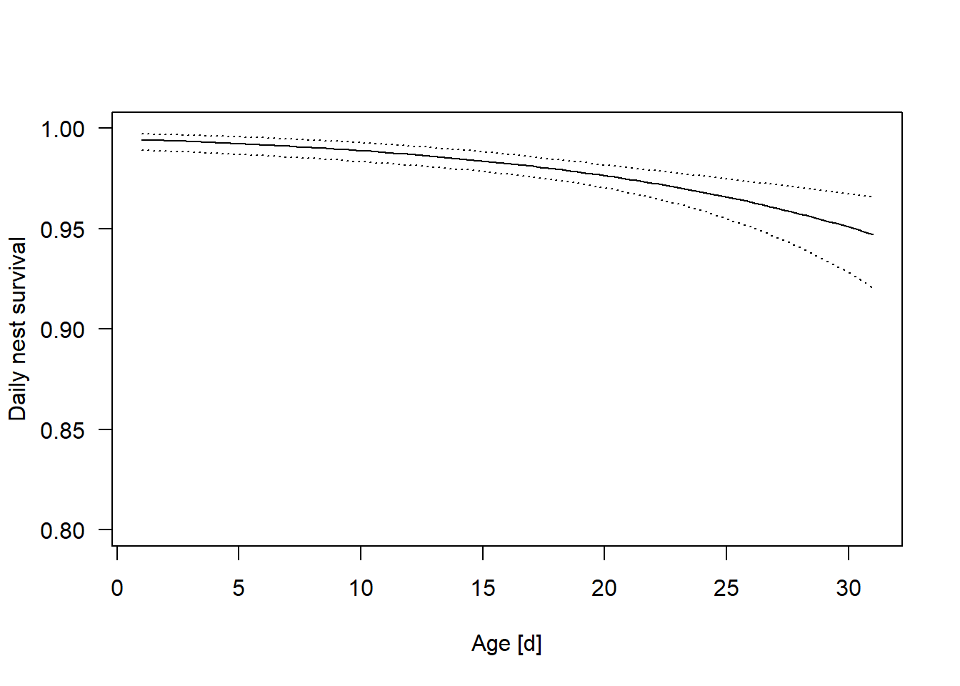

Figure 24.1: Estimated daily nest survival probability in relation to nest age. Dotted lines are 95% uncertainty intervals of the regression line.

24.8 Known fate model for irregular nest controls

When nest are controlled only irregularly, it may happen that a nest is found predated or dead after a longer break in controlling. In such cases, we know that the nest was predated or it died due to other causes some when between the last control when the nest was still alive and when it was found dead. In such cases, we need to tell the model that the nest could have died any time during the interval when we were not controlling.

To do so, we create a variable that indicates the time (e.g. day since first egg) when the nest was last seen alive (lastlive). A second variable indicates the time of the last check which is either the equal to lastlive when the nest survived until the last check, or it is larger than lastlive when the nest failure has been recorded. A last variable, gap, measures the time interval in which the nest failure occurred. A gap of zero means that the nest was still alive at the last control, a gapof 1 means that the nest failure occurred during the first day after lastlive, a gap of 2 means that the nest failure either occurred at the first or second day after lastlive.

# time when nest was last observed alive
lastlive <- apply(datax$y, 1, function(x) max(c(1:length(x))[x==1]))

# time when nest was last checked (alive or dead)
lastcheck <- lastlive+1 
# here, we turn the above data into a format that can be used for
# irregular nest controls. WOULD BE NICE TO HAVE A REAL DATA EXAMPLE!

# when nest was observed alive at the last check, then lastcheck equals lastlive
lastcheck[lastlive==datax$last] <- datax$last[lastlive==datax$last]

datax1 <- list(Nnests=datax$Nnests,
               lastlive = lastlive,
               lastcheck= lastcheck,
               first=datax$first,
               cover=datax$cover,
               age=datax$age,
               maxage=datax$maxage)
# time between last seen alive and first seen dead (= lastcheck)
datax1$gap <- datax1$lastcheck-datax1$lastlive

In the Stan model code, we specify the likelihood for each gap separately.

data {
  int<lower=0> Nnests;                // number of nests
  int<lower=0> lastlive[Nnests];      // day of last observation (alive)
  int<lower=0> lastcheck[Nnests];       // day of observed death or, if alive, last day of study 
  int<lower=0> first[Nnests];         // day of first observation (alive or dead)
  int<lower=0> maxage;                // maximum of last
  real cover[Nnests];                 // a covariate of the nest
  real age[maxage];                   // a covariate of the date
  int<lower=0> gap[Nnests];           // obsdead - lastlive
}

parameters {
  vector[3] b;                          // coef of linear pred for S
}

model {
  real S[Nnests, maxage-1];             // survival probability
                
  for(i in 1:Nnests){  
    for(t in first[i]:(lastcheck[i]-1)){ 
      S[i,t] = inv_logit(b[1] + b[2]*cover[i] + b[3]*age[t]); 
    }
  }

  // priors
  b[1]~normal(0,1.5);
  b[2]~normal(0,3);
  b[3]~normal(0,3);  

  // likelihood
  for (i in 1:Nnests) {
    for(t in (first[i]+1):lastlive[i]){
      1~bernoulli(S[i,t-1]);
    }
    if(gap[i]==1){
      target += log(1-S[i,lastlive[i]]);  // 
    }
    if(gap[i]==2){
      target += log((1-S[i,lastlive[i]]) + S[i,lastlive[i]]*(1-S[i,lastlive[i]+1]));  // 
    }
    if(gap[i]==3){
      target += log((1-S[i,lastlive[i]]) + S[i,lastlive[i]]*(1-S[i,lastlive[i]+1]) +
                    prod(S[i,lastlive[i]:(lastlive[i]+1)])*(1-S[i,lastlive[i]+2]));  // 
    }
    if(gap[i]==4){
      target += log((1-S[i,lastlive[i]]) + S[i,lastlive[i]]*(1-S[i,lastlive[i]+1]) +
                    prod(S[i,lastlive[i]:(lastlive[i]+1)])*(1-S[i,lastlive[i]+2]) +
                    prod(S[i,lastlive[i]:(lastlive[i]+2)])*(1-S[i,lastlive[i]+3]));  // 
    }

  }
}

# Run STAN
mod1 <- stan(file = "stanmodels/daily_nest_survival_irreg.stan", data=datax1, 
            chains=5, iter=2500, control=list(adapt_delta=0.9), verbose = FALSE)

Bayesian Data Analysis in Ecology with R and Stan