15 Generalized linear mixed models

---

15.1 Background

In chapter 13 on linear mixed effect models we have introduced how to analyze metric outcome variables for which a normal error distribution can be assumed (potentially after transformation), when the data have a hierarchical structure and, as a consequence, observations are not independent. In chapter 14 on generalized linear models we have introduced how to analyze outcome variables for which a normal error distribution can not be assumed, as for example binary outcomes or count data. More precisely, we have extended modelling outcomes with normal error to modelling outcomes with error distributions from the exponential family (e.g., binomial or Poisson). Generalized linear mixed models (GLMM) combine the two complexities and are used to analyze outcomes with a non-normal error distribution when the data have a hierarchical structure. In this chapter, we will show how to analyze such data. Remember, a hierarchical structure of the data means that the data are collected at different levels, for example smaller and larger spatial units, or include repeated measurements in time on a specific subject. Typically, the outcome variable is measured/observed at the lowest level but other variables may be measured at different levels. A first example is introduced in the next section.

15.2 Binomial mixed model

15.2.1 Background

To illustrate the binomial mixed model we use a subset of a data set used by Grüebler, Korner-Nievergelt, and Hirschheydt (2010) on barn swallow Hirundo rustica nestling survival (we selected a nonrandom sample to be able to fit a simple model; hence, the results do not add unbiased knowledge about the swallow biology!). For 63 swallow broods, we know the clutch size and the number of the nestlings that fledged. The broods came from 51 farms (larger unit), thus some of the farms had more than one brood. Note that each farm can harbor one or several broods, and the broods are nested within farms (as opposed to crossed, see chapter 13), i.e., each brood belongs to only one farm. There are three predictors measured at the level of the farm: colony size (the number of swallow broods on that farm), cow (whether there are cows on the farm or not), and dung heap (the number of dung heaps, piles of cow dung, within 500 m of the farm). The aim was to assess how swallows profit from insects that are attracted by livestock on the farm and by dung heaps. Broods from the same farm are not independent of each other because they belong to the same larger unit (farm), and thus share the characteristics of the farm (measured or unmeasured). Predictor variables were measured at the level of the farm, and are thus the same for all broods from a farm. In the model described and fitted below, we account for the non-independence of these clutches when building the model by including a random intercept per farm to model random variation between farms. The outcome variable is a proportion (proportion fledged from clutch) and thus consists of two values for each observation, as seen with the binomial model without random factors (Section 14.2.2): the number of chicks that fledged (successes) and the number of chicks that died (failures), i.e., the clutch size minus number that fledged.

The random factor “farm” adds a farm-specific deviation \(b_g\) to the intercept in the linear predictor. These deviations are modeled as normally distributed with mean \(0\) and standard deviation \(\sigma_g\).

\[ y_i \sim binomial\left(p_i, n_i\right)\\ logit\left(p_i\right) = \beta_0 + b_{g[i]} + \beta_1\;colonysize_i + \beta_2\;I\left(cow_i = 1\right) + \beta_3\;dungheap_i\\ b_g \sim normal\left(0, \sigma_g\right) \]

# Data on Barn Swallow (Hirundo rustica) nestling survival on farms
# (a part of the data published in Grüebler et al. 2010, J Appl Ecol 47:1340-1347)


library(blmeco)
data(swallowfarms)
#?swallowfarms # to see the documentation of the data set
dat <- swallowfarms
str(dat)

## 'data.frame':    63 obs. of  6 variables:
##  $ farm   : int  1001 1002 1002 1002 1004 1008 1008 1008 1010 1016 ...
##  $ colsize: int  1 4 4 4 1 11 11 11 3 3 ...
##  $ cow    : int  1 1 1 1 1 1 1 1 0 1 ...
##  $ dung   : int  0 0 0 0 1 1 1 1 2 2 ...
##  $ clutch : int  8 9 8 7 13 7 9 16 10 8 ...
##  $ fledge : int  8 0 6 5 9 3 7 4 9 8 ...

# check number of farms in the data set
length(unique(dat$farm))

## [1] 51

15.2.2 Fitting a binomial mixed model in R

15.2.2.1 Using the glmer function

dat$colsize.z <- scale(dat$colsize) # z-transform values for better model convergence
dat$dung.z    <- scale(dat$dung)
dat$die <- dat$clutch - dat$fledge
dat$farm.f <- factor(dat$farm)     # for clarity we define farm as a factor

The glmer function uses the standard way to formulate a statistical model in R, with the outcome on the left, followed by the ~ symbol, meaning “explained by”, followed by the predictors, which are separated by +. The notation for the random factor with only a random intercept was introduced in chapter 13 and is (1|farm.f) here.

Remember that for fitting a binomial model we have to provide the number of successful events (number of fledglings that survived) and the number of failures (those that died) within a two-column matrix that we create using the function cbind.

# fit GLMM using glmer function from lme4 package
library(lme4)
mod.glmer <- glmer(cbind(fledge,die) ~ colsize.z + cow + dung.z + (1|farm.f) , 
                   data=dat, 
                   family=binomial)

15.2.2.1.1 Assessing model assumptions for the glmer fit

The residuals of the model look fairly normal (top left panel of Figure 15.1 with slightly wider tails. The random intercepts for the farms look perfectly normal as they should. The plot of the residuals vs. fitted values (bottom left panel) shows a slight increase in the residuals with increasing fitted values. Positive correlations between the residuals and the fitted values are common in mixed models due to the shrinkage effect (chapter 13). Due to the same reason the fitted proportions slightly overestimate the observed proportions when these are large, but underestimate them when small (bottom right panel). What is looking like a lack of fit here can be seen as preventing an overestimation of the among farm variance based on the assumption that the farms in the data are a random sample of farms belonging to the same population.

The mean of the random effects is close to zero as it should. We check that because sometimes the glmer function fails to correctly separate the farm-specific intercepts from the overall intercept. A non-zero mean of random effects does not mean a lack of fit, but a failure of the model fitting algorithm. In such a case, we recommend using a different fitting algorithm, e.g. stan_glmer from the rstanarm package or brm from the brms package (see below).

A slight overdispersion (approximated dispersion parameter >1) seems to be present, but nothing to worry about.

par(mfrow=c(2,2), mar=c(3,5,1,1))    
# check normal distribution of residuals
qqnorm(resid(mod.glmer), main="qq-plot residuals")
qqline(resid(mod.glmer))

# check normal distribution of random intercepts
qqnorm(ranef(mod.glmer)$farm.f[,1], main="qq-plot, farm")
qqline(ranef(mod.glmer)$farm.f[,1])

# residuals vs fitted values to check homoscedasticity
plot(fitted(mod.glmer), resid(mod.glmer)) 
abline(h=0)

# plot data vs. predicted values
dat$fitted <- fitted(mod.glmer)
plot(dat$fitted,dat$fledge/dat$clutch)
abline(0,1)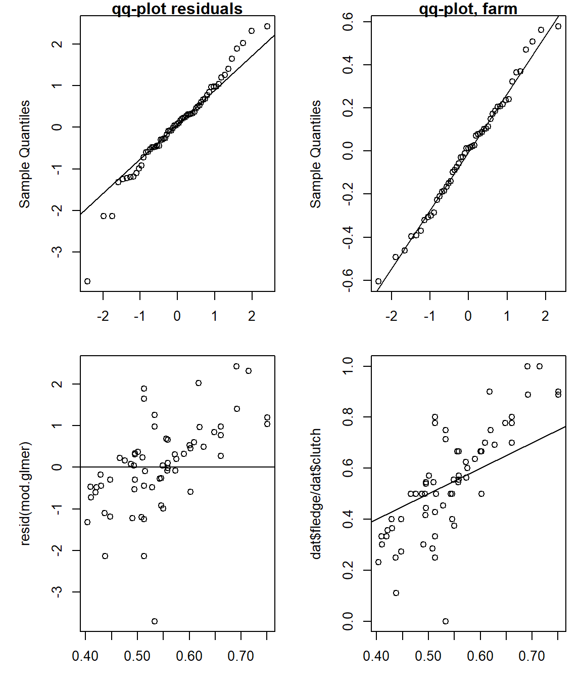

Figure 15.1: Diagnostic plots to assess model assumptions for “mod.glmer”. Upper left: quantile-quantile plot of the residuals vs. theoretical quantiles of the normal distribution. Upper right: quantile-quantile plot of the random effects “farm”. Lower left: residuals vs. fitted values. Lower right: observed vs. fitted values.

# check distribution of random effects
mean(ranef(mod.glmer)$farm.f[,1])

## [1] -0.001690303

# check for overdispersion
dispersion_glmer(mod.glmer)

## [1] 1.192931

Quite regularly, glmer returns a warning of non-convergence. In many such cases, it helps to simply set the argument control=glmerControl("bobyqa"). If it does not help, or if you get the message of a “boundary singular fit”, stan_glmer may be your solution: see the following chapter with more information.

15.2.2.2 Using rstanarm

A generalized linear mixed model can easily be fitted with the function stan_glmer from the package rstanarm. This can be particularly helpful, when glmer has some issues - situations we encounter more or less regularly are:

• When glmer does not converge and setting the argument control=glmerControl("bobyqa") does not help, stan_glmer might be able to fit the model.
• “boundary (singular) fit” warning from glmer: This usually means that a random factor variance cannot be estimated (it gets a value of 0, so do all levels of this random factor). This may signal that the variance is small and, hence, the random factor may not be so important. But we have also encountered situations where the variance was not negligible when fitting the same model with stan_glmer, so checking that out when you have “singular fit” is advisable.
• glmer cannot fit a binomial model with a factor that has a level (or several) with only 0s or only 1s (or, in the binomial case, only 0s or only values equal to the number of trials, e.g. 7 of 7, 4 of 4 etc.). stan_glmer, being Bayesian, can fit a model to such data. A factor level consisting of 4 0s (and no 1s) will have an estimate near 0 and a rather wide uncertainty, a factor level consisting of 40 0s (and no 1s) will also have an estimate near 0 but with a much narrower uncertainty.

In the following example we illustrate the second and third point using simulated data of a binary outcome variable (i.e. a binomial variable with number of trials = 1, also called a Bernoulli variable, and the model can be termed a logistic regression). There is one predictor: a factor called F1 with 5 levels. We also have a random factor called G.

set.seed(9)
library(rstanarm)
ddat <- expand.grid(F1 = rep(LETTERS[1:5],c(4,4,4,4,40))) # ddat, because the object dat from above will be used again below
ddat$G <- sample(letters[10:20],nrow(ddat),replace=T)   # just a dummy random factor to have for the glmer
tpe <- model.matrix(~F1,data=ddat) %*% runif(5,-1,1)    # true point estimate, generated using the matrix
   # model approach we also use when making effectplots from sim, explained most exhaustively in
   # the chapter on the simple linear regression
ddat$y <- rbinom(nrow(ddat),1,plogis(tpe))   # plogis is the inverse logit function

ddat$y[ddat$F1=="A"] <- 0
table(ddat$F1, ddat$y)  # note: factor level A has only 0s

##    
##      0  1
##   A  4  0
##   B  2  2
##   C  1  3
##   D  1  3
##   E 11 29

  # for the model fit, we don't estimate an intercept (by adding a "-1" in the formula), because we only
  # have one factor predictor - in this way we get an estimate for the mean of each factor level,
  # rather than an intercept (= estimate for baseline level) and 4 deviations from this for the other
  # 4 levels; both approaches are the same model, just with different parametrisation (different
  # "contrasts"), i.e. the coefficients have different meanings.
mod <- glmer(y ~ -1 + F1 + (1|G), data=ddat, family=binomial)
  # the model fits, only with the singular fit warning. But look at the standard errors:
summary(mod)

## Generalized linear mixed model fit by maximum likelihood (Laplace
##   Approximation) [glmerMod]
##  Family: binomial  ( logit )
## Formula: y ~ -1 + F1 + (1 | G)
##    Data: ddat
## 
##      AIC      BIC   logLik deviance df.resid 
##     73.6     85.7    -30.8     61.6       50 
## 
## Scaled residuals: 
##     Min      1Q  Median      3Q     Max 
## -1.7321 -1.0000  0.6159  0.6159  1.0000 
## 
## Random effects:
##  Groups Name        Variance Std.Dev.
##  G      (Intercept) 0        0       
## Number of obs: 56, groups:  G, 10
## 
## Fixed effects:
##       Estimate Std. Error z value Pr(>|z|)   
## F1A -3.112e+01  2.855e+06   0.000  0.99999   
## F1B  8.508e-08  1.000e+00   0.000  1.00000   
## F1C  1.099e+00  1.155e+00   0.951  0.34139   
## F1D  1.099e+00  1.155e+00   0.951  0.34139   
## F1E  9.694e-01  3.541e-01   2.738  0.00619 **
## ---
## Signif. codes:  0 '***' 0.001 '**' 0.01 '*' 0.05 '.' 0.1 ' ' 1
## 
## Correlation of Fixed Effects:
##     F1A   F1B   F1C   F1D  
## F1B 0.000                  
## F1C 0.000 0.000            
## F1D 0.000 0.000 0.000      
## F1E 0.000 0.000 0.000 0.000
## optimizer (Nelder_Mead) convergence code: 0 (OK)
## boundary (singular) fit: see help('isSingular')

Obviously something did not work! The problem is level A with only 0s. Also, the variance of the random factor G cannot be estimated, it “collapses” to 0 and throws the singluar fit warning. stan_glmer can fit this model. But let’s set all values from level E to 0, too.

ddat2 <- ddat
ddat2$y[ddat2$F1=="E"] <- 0
mod.rstanarm <- stan_glmer(y ~ -1 + F1 + (1|G), data=ddat2, family=binomial, refresh=0)
summary(mod.rstanarm)[c(1:5,16),] %>% round(2)

##                                   mean mcse   sd    10%   50%   90% n_eff Rhat
## F1A                              -8.93 0.11 5.61 -16.82 -7.78 -2.69  2651    1
## F1B                              -0.05 0.02 1.39  -1.79 -0.05  1.64  3180    1
## F1C                               1.62 0.03 1.76  -0.36  1.42  3.85  2862    1
## F1D                               1.83 0.03 1.72  -0.16  1.64  4.01  2439    1
## F1E                              -7.37 0.05 2.73 -11.10 -6.86 -4.30  2885    1
## Sigma[G:(Intercept),(Intercept)]  1.95 0.10 3.63   0.01  0.56  5.23  1456    1

The model fits without problem, all R-hat are good (remember: they should be near 1, ideally <1.1, 18), coefficient estimates make sense (they are on the logit scale, of course). Both estimates for A and E are strongly negative, i.e. inverse-logit of these are close to 0, and the uncertainty for A is a bit larger than for E, which makes sense since E has many more 0s than A. Also, the standard deviation for the random factor G can now be estimated - and check it out, it is not extremely small!

The point estimates with 95% compatibility intervals for the 5 means are:

 # we generate a newdat. We want to have each level of F1. And we want to be sure that the level
 # order is the same as in ddat2 by setting the argument "levels" to levels(ddat2$F1). When the
 # factor levels are ordered alpha-numerically (as in our case) this would not be needed, but if
 # they have a custom order, forgetting to set the order in newdat equal to the orde in ddat2 will have
 # catastrophic consequences (estimates and factor levels would be mixed up)
newdat <- data.frame(F1 = factor(levels(ddat2$F1),levels=levels(ddat2$F1)))
 # now we can use posterior_epred, with the argument re.form=NA to not estimate for random factors
fitmat <- posterior_epred(mod.rstanarm, newdata=newdat, re.form=NA)

newdat$fit <- apply(fitmat,2,mean)
newdat$lwr <- apply(fitmat,2,quantile,probs=0.025)
newdat$upr <- apply(fitmat,2,quantile,probs=0.975)

The effectplot can now easily be plotted (here a R base code, of course you can also ggplot it)

set.seed(43)  # just for the jitter
newdat$x <- 1:nlevels(newdat$F1)
plot(jitter(as.numeric(ddat2$F1),amount=0.07)+0.3,jitter(ddat2$y,amount=0.05),pch=21,bg=as.numeric(ddat2$F1),
     xlim=c(0.5,nlevels(ddat2$F1)+0.5), las=1, ylab="y (raw data) and probability", xlab="F1", xaxt="n")
axis(1,1:5,levels(newdat$F1),tick=F)
newdat$x <- 1:nlevels(newdat$F1)
segments(newdat$x,newdat$lwr, newdat$x,newdat$upr, lwd=1)
points(newdat$x, newdat$fit, pch=21, cex=1.3, bg=newdat$x)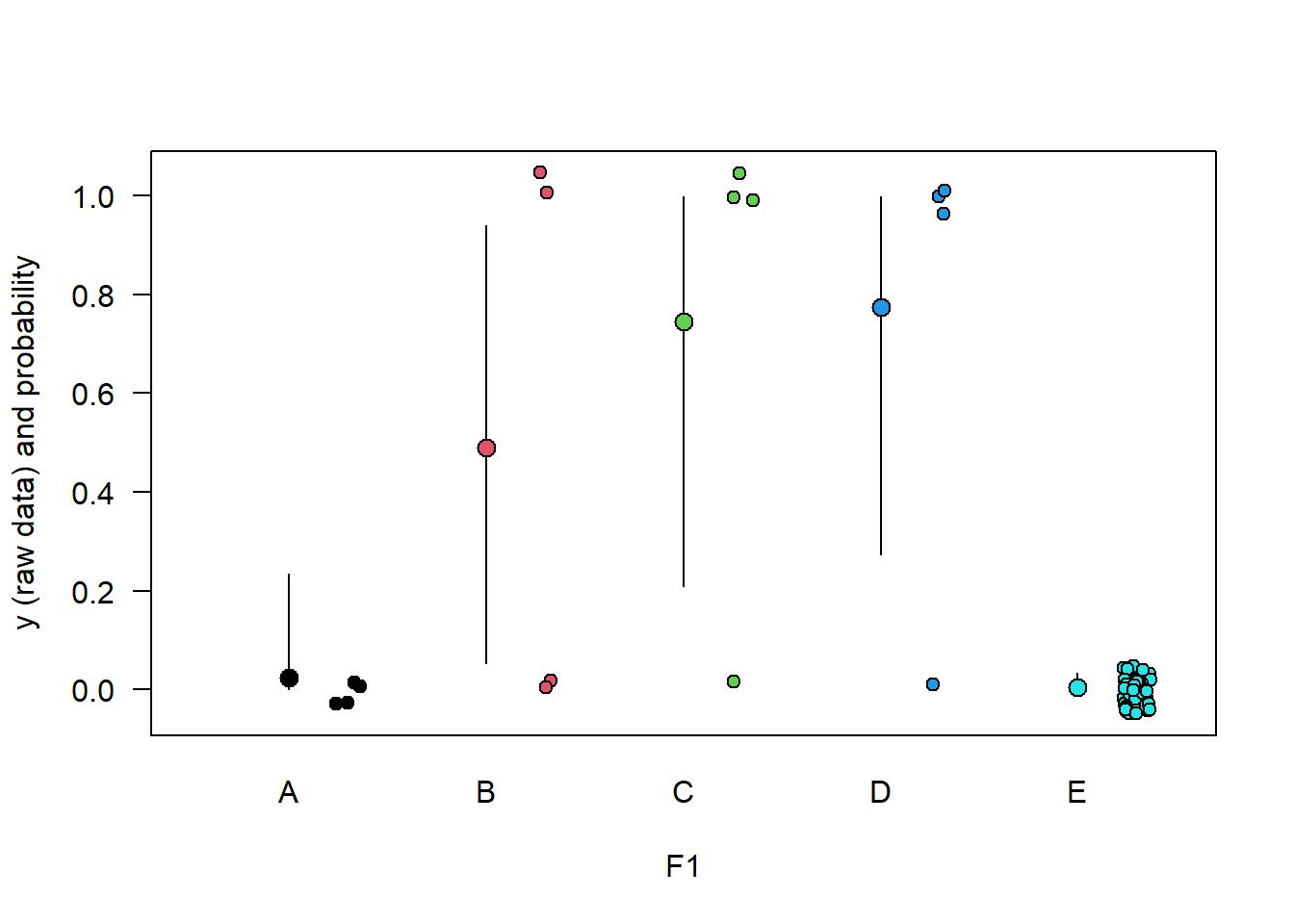

Figure 5.2: Raw data (points, jittered to reduce overlap) and estimated means with 95% compatiblity interval for data from 5 groups A-E and a binary outcome variable y (0/1). Groups A and E have only 0s.

The estimates for groups B-D are uncertain, due to the small sample size for each of them. The mean of groups A and E are estimated to be near 0, with much more certainty for E that it is really most likely very small. Estimates and compatibility intervals are bound between 0 and 1, which makes sense for a probability, and which is achieved by using a logit link function in the binomial model.

15.2.2.3 Using the brm function

We have introduced brm from the brms package in Chapter 11.1.2.4.

In the case of a binomial outcome, the notation for brm is different from the notation in e.g. glmer: in brm, the binomial outcome is specified in the format successes|trials(), which is the number of fledged nestlings out of the total clutch size in our case. In contrast, the glmer function required to specify the number of nestlings that fledged and died (which together sum up to clutch size), in the format cbind(successes, failures).

The family is also called binomial in brm, but would be bernoulli for a binary outcome, whereas glmer uses binomial in both situations (Bernoulli distribution is a special case of the binomial). However, it is slightly confusing that (at the time of writing this chapter) the documentation for brmsfamily does not mention the binomial family under Usage, where it probably went missing, but it is mentioned under Arguments for the argument family.

In Chapter 11.1.2.4 we also shortly treat the priors of brm. In many practical cases, we simply use the default priors, which we can request using the function get_prior with the same arguments as we use for brm itself. In the case of more complex models, especially with a logit link function, it may at times help to provide slightly more informative priors for the effect sizes (the class b priors in the output from get_prior) than flat priors. We do that in our case, also to illustrate how priors can be specified by the function prior.

library(brms)

# check which parameters need a prior
get_prior(fledge|trials(clutch) ~ colsize.z + cow + dung.z + (1|farm.f), 
          data=dat, 
          family=binomial(link="logit"))

##                 prior     class      coef  group resp dpar nlpar lb ub tag
##                (flat)         b                                           
##                (flat)         b colsize.z                                 
##                (flat)         b       cow                                 
##                (flat)         b    dung.z                                 
##  student_t(3, 0, 2.5) Intercept                                           
##  student_t(3, 0, 2.5)        sd                                   0       
##  student_t(3, 0, 2.5)        sd           farm.f                  0       
##  student_t(3, 0, 2.5)        sd Intercept farm.f                  0       
##        source
##       default
##  (vectorized)
##  (vectorized)
##  (vectorized)
##       default
##       default
##  (vectorized)
##  (vectorized)

# specify own priors
myprior <- prior(normal(0,5), class="b")
             
# as before, we save the compiled model, just to speed up the rendering of the book - 
# in analyses, you may or may not store the compiled model.

# mod.glmm.brm <- brm(fledge|trials(clutch) ~ colsize.z + cow + dung.z + (1|farm.f) , 
#                data=dat, family=binomial(link="logit"),
#                prior=myprior, chains = 0)
# save(mod.glmm.brm, file="RData/mod.glmm.brm.RData")
load("RData/mod.glmm.brm.RData")
mod.brm <- update(mod.glmm.brm,
               warmup = 500, 
               iter = 2000, 
               chains = 2,
               init = "random", 
               cores = 2,
               seed = 123)
# note: thin=1 is default and we did not change this here.

15.2.2.3.1 Checking model fit by posterior predictive model checking

To assess how well the model fits to the data we do posterior predictive model checking (Chapter 16). For binomial as well as for Poisson models comparing the standard deviation of the data with those of replicated data from the model is particularly important. If the standard deviation of the real data would be much higher compared to the ones of the replicated data from the model, overdispersion would be an issue. However, here, the model is able to capture the variance in the data correctly (Figure 15.2). The fitted vs observed plot also shows a good fit.

yrep <- posterior_predict(mod.brm)
sdyrep <- apply(yrep, 1, sd)

par(mfrow=c(1,3), mar=c(3,4,1,1))
hist(yrep, freq=FALSE, main=NA, xlab="Number of fledglings")
hist(dat$fledge, add=TRUE, col=rgb(1,0,0,0.3), freq=FALSE)
legend(10, 0.15, fill=c("grey",rgb(1,0,0,0.3)), legend=c("yrep", "y"))

hist(sdyrep)
abline(v=sd(dat$fledge), col="red", lwd=2)

plot(fitted(mod.brm)[,1], dat$fledge, pch=16, cex=0.6)
abline(0,1)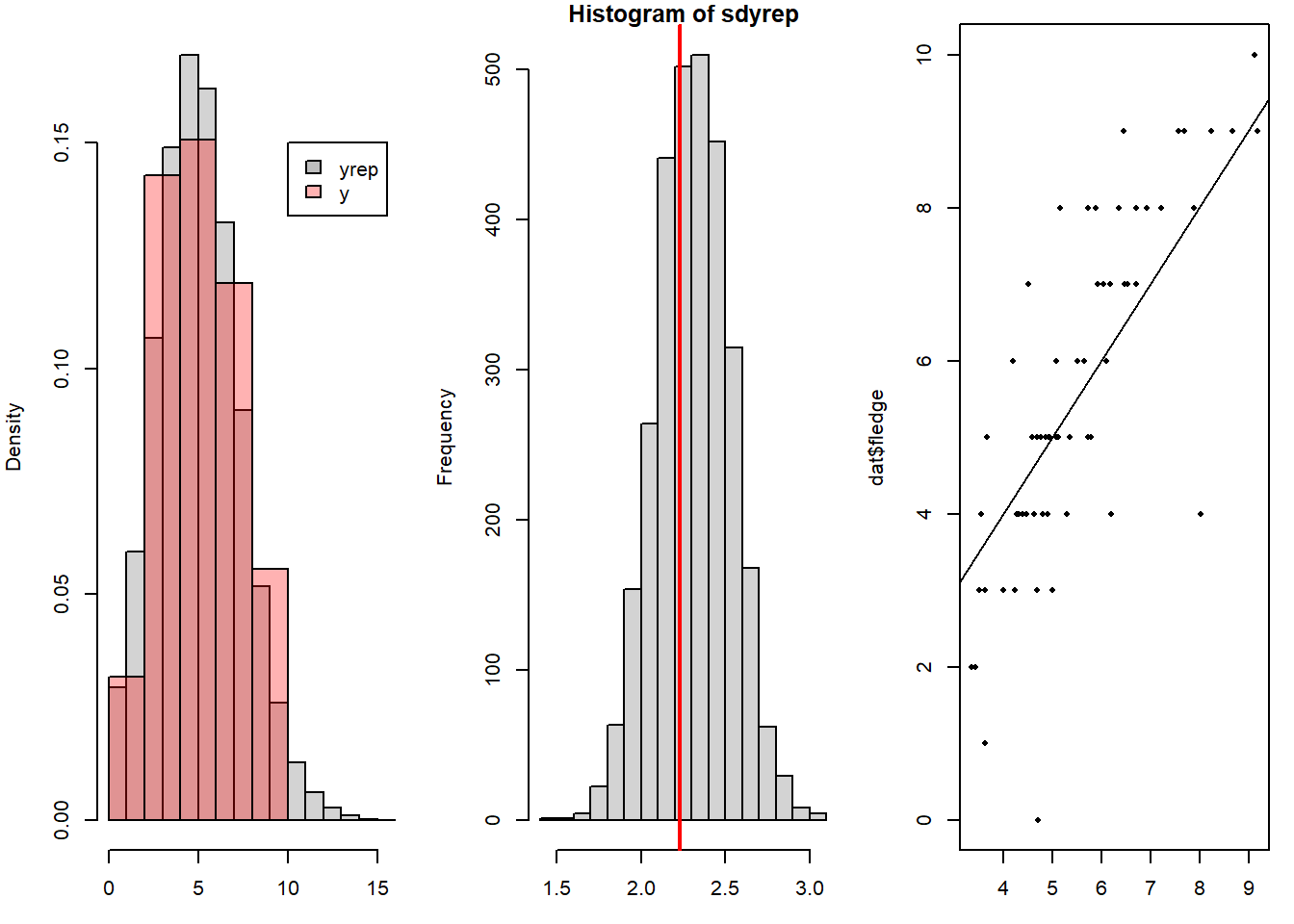

Figure 15.2: Posterior predictive model checking: Histogram of the number of fledglings simulated from the model together with a histogram of the real data, and a histogram of the standard deviations of replicated data from the model together with the standard deviation of the data (vertical line in red). The third plot gives the fitted vs. observed values.

Another classical question we can address using posterior predictive model checking is whether we have zero-inflation, i.e. whether the data has more zeros than the model predicts. In our example, there is only one Zero among 63 data rows, hence this is certainly not an issue. Nevertheless, we provide the code how this could be checked (analogous to checking the standard deviation done above).

Zeroyrep <- apply(yrep, 1, FUN=function(x)sum(x==0))   # count the nr of zeros in each replicate data
hist(Zeroyrep, xlab="Nr of zeros", xlim=range(c(Zeroyrep,sum(dat$fledge==0))))
abline(v=sum(dat$fledge==0), col="red", lwd=2)
  # the red line should not be far outside the gray histogram; the xlim used in the histogram
  # makes sure that the red line will be visible in the plot, because sometimes it can be far
  # away from the histogram (which would show that the model is not great regarding Zeros)

After checking the diagnostic plots, the posterior predictive model checking and the general model fit, we assume that the model describes the data generating process reasonably well, so that we can proceed to make inferences from the model.

15.2.3 Presenting the results

The generic summary function gives us the results for the model object containing the fitted model, and works for both the model fitted with glmer and brm. Let’s start having a look at the summary from mod.glmer. The summary provides the fitting method, the model formula, statistics for the model fit including the Akaike information criterion (AIC), the Bayesian information criterion (BIC), the scaled residuals, the random effects variance and information about observations and groups, a table with coefficient estimates for the fixed effects (with standard errors and a z-test for the coefficient) and correlations between fixed effects. We recommend to always check if the number of observations and groups, i.e., 63 barn swallow nests from 51 farms here, is correct. This information shows if the glmer function has correctly recognized the hierarchical structure in the data. Here, this is correct. To assess the associations between the predictor variables and the outcome analyzed, we need to look at the column “Estimate” in the table of fixed effects. This column contains the estimated model coefficients, and the standard error for these estimates is given in the column “Std. Error”, along with a z-test for the null hypothesis of a coefficient of zero. In the random effects table, the among farm variance and standard deviation (square root of the variance) are given. The function confint shows the 95% confidence intervals for the random effects (.sig01) and fixed effects estimates.

In the summary output from mod.brm we see the model formula and some information on the Markov chains after the warm-up. In the group-level effects (between group standard deviations) and population-level effects (effect sizes, model coefficients) tables some summary statistics of the posterior distribution of each parameter are given. The “Estimate” is the mean of the posterior distribution, the “Est.Error” is the standard deviation of the posterior distribution (which is the standard error of the parameter estimate). Then we see the lower and upper limit of the 95% credible interval. Also, some statistics for measuring how well the Markov chains converged are given: the “Rhat” and the effective sample size (ESS). The bulk ESS tells us how many independent samples we have to describe the posterior distribution, and the tail ESS tells us on how many samples the limits of the 95% credible interval is based on.

Because we used the logit link function, the coefficients are actually on the logit scale and are a bit difficult to interpret. What we can say is that positive coefficients indicate an increase and negative coefficients indicate a decrease in the proportion of nestlings fledged. For continuous predictors, as colsize.z and dung.z, this coefficient refers to the change in the logit of the outcome with a change of one in the predictor (e.g., for colsize.z an increase of one corresponds to an increase of a standard deviation of colsize). For categorical predictors, the coefficients represent a difference between one category and another (reference category is the one not shown in the table). To visualize the coefficients we could draw effect plots.

# glmer
summary(mod.glmer)

## Generalized linear mixed model fit by maximum likelihood (Laplace
##   Approximation) [glmerMod]
##  Family: binomial  ( logit )
## Formula: cbind(fledge, die) ~ colsize.z + cow + dung.z + (1 | farm.f)
##    Data: dat
## 
##      AIC      BIC   logLik deviance df.resid 
##    282.5    293.2   -136.3    272.5       58 
## 
## Scaled residuals: 
##     Min      1Q  Median      3Q     Max 
## -3.2071 -0.4868  0.0812  0.6210  1.8905 
## 
## Random effects:
##  Groups Name        Variance Std.Dev.
##  farm.f (Intercept) 0.2058   0.4536  
## Number of obs: 63, groups:  farm.f, 51
## 
## Fixed effects:
##             Estimate Std. Error z value Pr(>|z|)  
## (Intercept) -0.09533    0.19068  -0.500   0.6171  
## colsize.z    0.05087    0.11735   0.434   0.6646  
## cow          0.39370    0.22692   1.735   0.0827 .
## dung.z      -0.14236    0.10862  -1.311   0.1900  
## ---
## Signif. codes:  0 '***' 0.001 '**' 0.01 '*' 0.05 '.' 0.1 ' ' 1
## 
## Correlation of Fixed Effects:
##           (Intr) clsz.z cow   
## colsize.z  0.129              
## cow       -0.828 -0.075       
## dung.z     0.033  0.139 -0.091

confint.95 <- confint(mod.glmer); confint.95

##                   2.5 %    97.5 %
## .sig01       0.16809483 0.7385238
## (Intercept) -0.48398346 0.2863200
## colsize.z   -0.18428769 0.2950063
## cow         -0.05360035 0.8588134
## dung.z      -0.36296714 0.0733620

# brm
summary(mod.brm)

##  Family: binomial 
##   Links: mu = logit 
## Formula: fledge | trials(clutch) ~ colsize.z + cow + dung.z + (1 | farm.f) 
##    Data: dat (Number of observations: 63) 
##   Draws: 2 chains, each with iter = 2000; warmup = 500; thin = 1;
##          total post-warmup draws = 3000
## 
## Multilevel Hyperparameters:
## ~farm.f (Number of levels: 51) 
##               Estimate Est.Error l-95% CI u-95% CI Rhat Bulk_ESS Tail_ESS
## sd(Intercept)     0.55      0.16     0.26     0.86 1.00      910     1284
## 
## Regression Coefficients:
##           Estimate Est.Error l-95% CI u-95% CI Rhat Bulk_ESS Tail_ESS
## Intercept    -0.10      0.21    -0.52     0.32 1.00     2863     2165
## colsize.z     0.05      0.14    -0.21     0.34 1.00     2266     1794
## cow           0.41      0.25    -0.06     0.90 1.00     3069     2117
## dung.z       -0.15      0.12    -0.38     0.09 1.00     3254     2241
## 
## Draws were sampled using sampling(NUTS). For each parameter, Bulk_ESS
## and Tail_ESS are effective sample size measures, and Rhat is the potential
## scale reduction factor on split chains (at convergence, Rhat = 1).

From the results we conclude that in farms without cows (when cow=0) and for average colony sizes (when colsize.z=0) and average number of dung heaps (when dung.z=0) the average nestling survival of Barn swallows is the inverse-logit function of the Intercept, thus, plogis(-0.1) = 0.47 with a 95% uncertainty interval of 0.37 - 0.58. We further see that colony size and number of dung heaps are less important than whether cows are present or not. Their estimated partial effect is small and their uncertainty interval includes only values close to zero. However, whether cows are present or not may be important for the survival of nestlings. The average nestling survival in farms with cows is plogis(-0.1+0.41) = 0.58. For getting the uncertainty interval of this survival estimate, we need to do the calculation for every simulation from the posterior distribution of both parameters.

bsim <- posterior_samples(mod.brm)
# survival of nestlings on farms with cows:
survivalest <- plogis(bsim$b_Intercept + bsim$b_cow)
quantile(survivalest, probs=c(0.025, 0.975)) # 95% uncertainty interval

##      2.5%     97.5% 
## 0.5126716 0.6412675

In medical research, it is standard to report the fixed-effects coefficients from GLMM with binomial or Bernoulli error as odds ratios by taking the exponent (R function exp for \(e^{()}\)) of the coefficient on the logit-scale. For example, the coefficient for cow from mod.glmer, 0.39 (95% CI from -0.05 to -0.05), represents an odds ratio of exp( 0.39)=1.48 (95% CI from 0.95 to 0.95). This means that the odds for fledging (vs. not fledging) from a clutch from a farm with livestock present is about 1.5 times larger than the odds for fledging if no livestock is present (relative effect).

15.3 Poisson mixed model

15.4 Summary