5 Transformations
Transformations of predictors (and sometimes also of the outcome variable) are very common. There is nothing “fishy” about transformations - not transforming a predictor is as much a decision as making e.g. a log-transformation. The aim is not to conjure some non-existing effects. If a predictor shows an effect after transformation, this means that the nature of the relationship simply is on this transformed scale; if a predictor has a multiplicative effect on the outcome variable, we will find a linear relationship between the outcome variable and the log-transformed predictor. Without transformation, the model would violate the assumption of “identically distributed” data around the regression line, only the transformation makes the model valid.
When we use a transformation, we can still make effectplots (our favorite way to present the results) on the original scale. Or, we can plot on the transformed (e.g. log) scale; which one is better is not a statistical question, rather we should think about which version best conveys the biological (or other topical) meaning of our results.
We can distinguish two different types of transformations which have fundamentally different motivations and consequences.
Linear transformations
Linear transformations have no effect on the model performance itself: the variance explained by the model remains the same, effectplots don’t change. The motivation is not to achieve a better fit of the model to the data, but to a) facilitate model convergence and to b) improve the interpretability of model coefficients. The most commonly used linear transformation is centering and scaling (which can be called the “z-transformation”), for details see below. Complex models (e.g. those fitted with glmer, but often also simpler models) may not converge if you don’t apply a z-transformation to the linear predictors, especially when the predictor on the original scale has large values. For the same reason, when we want to include a polynomial term in the model, we usually use orthogonal rather than raw polynomials (polynomials are not linear transformations, but orthogonal polynomials are linear compared to raw polynomials). b) Coefficients of z-transformed predictors and of orthogonal polynomials have a more natural interpretation - discussed in the corresponding chapters below.
Non-linear transformations The most commonly used non-linear transformations include the logarithm (usually just called log-transformation), polynomials (of degree 2 and more), the square-root, the arcussinus-squre-root (arcsin-square-root) and the logit. They have an effect on the model fit and will change the effectplot compared to using the untransformed predictor. E.g., when fitting a normal linear regression, the regression line will not be straight any more. The aim of these transformations is to improve model fit, i.e. to better capture the relationships that are in the data.
Non-linear transformations allow the use of the linear modeling framework even if the true nature of a relationship is not linear - to the degree that it can be represented by one of the available transformations. If the relationship is “very non-linear”, such as a complex phenology (activity of an organism over the year, with date as predictor), the effect of the predictor can be estimated using a smoother. In that case, we talk of a generalized additive model (GAM; actually, even GAM are linear models in their mathematical structure).
Note that transformations generally are only done for continuous predictors (= a covariable). However, sometimes, we may convert a (ordered) factor to a covariable, which can be seen as a type of transformation. This is discussed in a following chapter, together with the inverse: categorizing a covariable.
5.1 Some R-specific aspects
A transformation on a predictor can be calculated and stored as a new variable in the data object:
dat <- data.frame(a = runif(20,2,6),
                  b = rnorm(20,2,100))                           # some simulated data
dat$y <- rnorm(20,2-0.6*log(dat$a)-0.12*dat$b+0.003*dat$b^2,11)  # simulated outcome variable
dat$a.l <- log(dat$a)    # the log of x is stored in the new variable $x.l
dat$b.z <- scale(dat$b)  # the variable b is centerd and scaled to 1 SD by the function scale, and stored in $b.z
Then, the variable (“a.l”, “b.z”) can be used in the model just like any variable.
Alternatively, transformations can be done directly in the model formula:
mod1 <- lm(y ~ log(a), data=dat)     # the effect of the log of a on b is estimated
mod2 <- lm(y ~ b + I(b^2), data=dat) # using a linear and quadratic effect
  # as dat$b has large values, better use scaled dat$b, i.e. dat$b.z:
mod3 <- lm(y ~ b.z + I(b.z^2), data=dat)  # the I() makes that first the square is calculated, then these values are used
  # or, even better, especially for complex models, use orthogonal polynomials by applying the function poly
mod4 <- lm(y ~ poly(b,2), data=dat)   # the "2" asks for 2 polynomials, i.e. linear and quadratic
Models 2 to 4 are all the same model in the sense that they create the same effectplot.
Beware: It is often nice to z-transform the orthogonal polynomials. For that, we cannot use a double-function in the formula notation, rather the polynomials have to be created before the modeling, stored as a new variable, and only the z-transformation can be done in the formula (or outside, too, if you prefer). We get back to this in the polynomial chapter below.
5.2 First-aid transformations
J. W. Tukey termed the following three transformations the “first aid transformations”:
- log-transformation for concentrations and amounts
- square-root transformation for count data
- arcsin-square-root transformation for proportions (
asin(sqrt(dat$x)))
Werner Stahel, a pivotal stats teacher for several of us, provides this information in his (german) book Stahel (2000). In our experience, the log-transformation can often be helpful, especially for strongly right skewed positive variables. We don’t often use the square-root transformation, but every now and then the arcsin-square-root transformation.
5.3 Log-transformation with Stahel
Log-transformations are often used and often very helpful, especially, as stated above, for strongly right skewed positive variables. Without the transformation, the large values, far away from the bulk of data, may have an unduely strong effect on the regression line (leading to a large “Cook’s distance”, see 12).
When log-transforming a predictor, we model its multiplicative effect on the outcome variable, while without transformation, it is the additive effect. This means: The model assumes that multiplying x by a factor F increases y by amount G (rather than increasing x by amount F increases y by amount G for the additive case). It seems that right skewed variables often relate in a multiplicative way to the outcome variable (for reasons that may lie in the heart of how mathematics works in our universe - we don’t know). But it is a good that down-scaling large values and changing to a multiplicative effect often both increase the model fit, else the log-transformation would not be that useful.
The log-transformation is great, as long as there are no zeros (and, of course, it does not work with negative values at all), as the log of 0 is minus infinity. But in real life, we often have zeros, and then, many people just add 1 to the values before log-transformation. This can be ok, but it is not optimal when the (non-zero) values are small. For that reason, some suggest to add 0.5 times the smallest non-zero value. Rob J Hyndman also presents the Box-Cox transformation in a blog, which apparently can be done using the R function log1p.
We made good experience with a transformation suggested by our above mentioned stats teacher Werner Stahel in his book (Stahel 2000): log(x + c), and c is the squared 25% quantile of the non-zero values divided by the 75% quantile of the non-zero values. This performs well with zeros, but is also much better than adding 1 in many cases, e.g. when there are many very small values.
set.seed(3)
x <- exp(runif(200,-3,5))  # a strongly skewed variable
x[sample(1:length(x),7)] <- 0   # put some values to exactly 0
x2 <- x/1000   # small values

# our custom function to calculate the Stahel-constant:
stahelc <- function(x) {
  ix <- x>0
  return((quantile(x[ix],0.25,na.rm=T))^2/quantile(x[ix],0.75,na.rm=T))
}par(mfrow=c(2,4), mar=c(2,1,1,1), oma=c(0,2,1,0))
hist(x, nclass=30, main="raw values", xlab="", ylab="", yaxt="n")
mtext("larger values",2,1,xpd=NA)
hist(log(x+1), nclass=30, main="+1", xlab="", ylab="", yaxt="n")
hist(log(x+stahelc(x)), nclass=30, main="Stahel", xlab="", ylab="", yaxt="n")
hist(log1p(x), nclass=30, main="Box-Cox", xlab="", ylab="", yaxt="n")
hist(x2, nclass=30, main="raw values", xlab="", ylab="", yaxt="n")
mtext("small values",2,1,xpd=NA)
hist(log(x2+1), nclass=30, main="+1", xlab="", ylab="", yaxt="n")
hist(log(x2+stahelc(x2)), nclass=30, main="Stahel", xlab="", ylab="", yaxt="n")
hist(log1p(x2), nclass=30, main="Box-Cox", xlab="", ylab="", yaxt="n")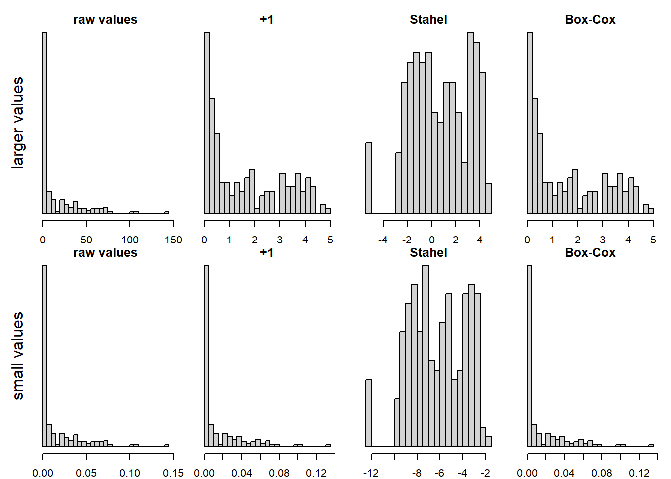
Figure 5.1: log-transformation of an original variable (leftmost two panels), for a variable with larger values (above row of panels) and one with smaller values (lower row). Adding 1 or the Box-Cox transformation don’t seem to help much, adding a constant according to Stahel performs best in these cases.
5.11 Identity transformation
This simply means the transformation to itself, i.e. no transformation. We only list this here because, sometimes, we read about the “identity link” in the context of generalize linear models (Chapter @glm), where a link function is used (e.g. log-link function for Poisson models). Normal linear models (@lm) are a special case of generalize linear models, namely a Gauss (or “normal”) model with an identity-link function.
5.12 Transformations on the outcome variable
Transformations can also be made on the outcome variable. A very skewed outcome variable may be log-transformed. If the outcome variable is a proportion (e.g. the proportion of survivors from a nest, and we don’t have the actual number of survivors and non-survivors - if we have these numbers, we would fit a binomial model 14), the arcsin-square-root transformation can be meaningful.
But remember to back-transform predictions, if you want to give them on the original scale!